Recall and Quarantine Scope vs Traceability Resolution: Lot Tracking Compared with Cell-Plus-Parameter Tracking
Abstract
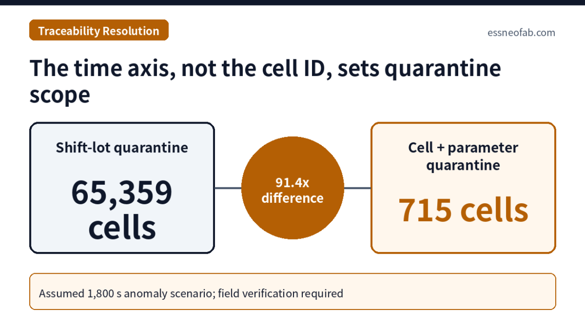
On an assumed line producing 25,000,000 cells per year, a process anomaly lasting 1,800 s at one station leads to a quarantine population of 196,078 cells at lot level (production-day lot plus adjacent lot), 65,359 cells at shift-lot level, 2,159 cells with cell-to-tray mapping, 2,045 cells with per-cell timestamps, and 715 cells with per-cell process-parameter linkage. The main lever that narrows the quarantine scope by roughly 30× is not the cell ID itself but time-axis resolution (lot → tray); per-cell parameter linkage narrows it by a further ~2.9×. Under 10-year retention, storage cost is below 0.1% of the quarantine cost of a single anomaly at shift-lot level, so the real trade-off variables for resolution investment are integration cost and anomaly frequency, not storage volume. All figures are an assumed scenario and require field verification.
1. Conclusion First — The Time Axis, Not the ID, Determines Quarantine Scope
When traceability[1] resolution is raised, the step at which the quarantine[2] scope collapses is the transition from “lot” to “time-stamped tray”; adding a cell ID on top of that yields only about 5.6%. The second large gain of cell-level tracking comes not from the ID but from linkage to process-parameter values.
Situation (S): When a process anomaly is detected, a cell line fixes the anomaly time window through backward trace[3], quarantines the cells in that window, and decides on re-inspection or scrapping. Complication (C): Many lines still set this scope from lot genealogy, and cell-level tracking is deferred on data-cost grounds. Question (Q): By how many times does the quarantine scope change at each resolution step, and where is the balance point against data cost? Answer (A): The lot → tray transition narrows it by about 30×, cell-parameter linkage by about 2.9×, and storage cost does not become a decision variable.
Public recall notices also show that identifier resolution defines scope. On 16 December 2020 the U.S. Consumer Product Safety Commission (CPSC) announced a recall of about 1,815 LG Chem RESU 10H residential ESS units identified by the serial-number prefix “R15563P3SSEG”, and on 4 August 2021 it announced an additional recall of about 10,000 units identified by the prefix “R15563P3” (cumulative about 11,815 units, about 6.5× the first notice). This article makes no judgement on the cause of that recall; it cites only the structure that the resolution of the identifier disclosed externally sets the lower bound of the quarantine scope.
2. Mechanism — Five Resolution Levels and Quarantine Rules
The assumed line produces 100 Ah, 3.2 V cells (0.32 kWh) at a capacity of 8 GWh/year, i.e., 25,000,000 cells per year. With available operating time set at 22,032,000 s/year (300 days × 86,400 s × 85%, assumed), takt time[4] is 22,032,000 ÷ 25,000,000 = 0.881 s/cell and line output is about 1.135 cells/s. About 2,042 cells actually pass the station during the 1,800 s anomaly window.
The quarantine rule differs by resolution. At lot level, the lot containing the anomaly is quarantined together with one adjacent lot that may be mixed through inter-process buffer[5] flow. Levels with time records add a guard band[6] equal to the time-alignment error around the anomaly window, and levels with linked parameter values quarantine only cells within the window that actually exceeded the control limit or fall within the boundary margin.
| Resolution level | Linked data | Backward-trace unit | Annual data volume (assumed) | 10-year retention total |
|---|---|---|---|---|
| L1 Production-day lot | Material lot ↔ production lot genealogy | 86,400 s | about 18 MB | about 0.18 GB |
| L2 Shift lot | L1 + shift split | 28,800 s | about 55 MB | about 0.55 GB |
| L3 Cell-tray mapping | Cell serial ↔ tray ID, per-tray station time (time error ±30 s) | Tray (24 cells, about 21 s) | about 10 GB | about 100 GB |
| L4 Per-cell timestamps | Pass time at 20 stations per cell ID (synchronised ±1 s) | Cell (0.881 s) | about 75 GB | about 750 GB |
| L5 Cell + process parameters | L4 + about 40 parameter values per station | Cell and parameter value | about 275 GB | about 2.75 TB |
The data volume in Table 1 grows by one or two orders of magnitude per level, but even at L5 the absolute amount is about 2.75 TB after 10 years. Resolution discussions often start from the premise that “there is too much data”, yet excluding waveforms, the tracking data of a single cell line does not fall into the big-data category.
3. Calculation — Quarantined Cells by Resolution
| Resolution level | Quarantine rule | Quarantined cells | Multiple of L5 | Quarantine cost per anomaly (assumed) |
|---|---|---|---|---|
| L1 Production-day lot | Anomaly lot + 1 adjacent lot | 196,078 cells | 274.3× | about KRW 3.92 billion |
| L2 Shift lot | Anomaly lot + 1 adjacent lot | 65,359 cells | 91.4× | about KRW 1.31 billion |
| L3 Cell-tray mapping | (1,800 s + guard band 60 s) + 2 boundary trays | 2,159 cells | 3.0× | about KRW 43 million |
| L4 Per-cell timestamps | 1,800 s + guard band 2 s | 2,045 cells | 2.9× | about KRW 41 million |
| L5 Cell + process parameters | Out-of-limit and boundary cells in window (35%, assumed) | 715 cells | 1.0× | about KRW 14 million |
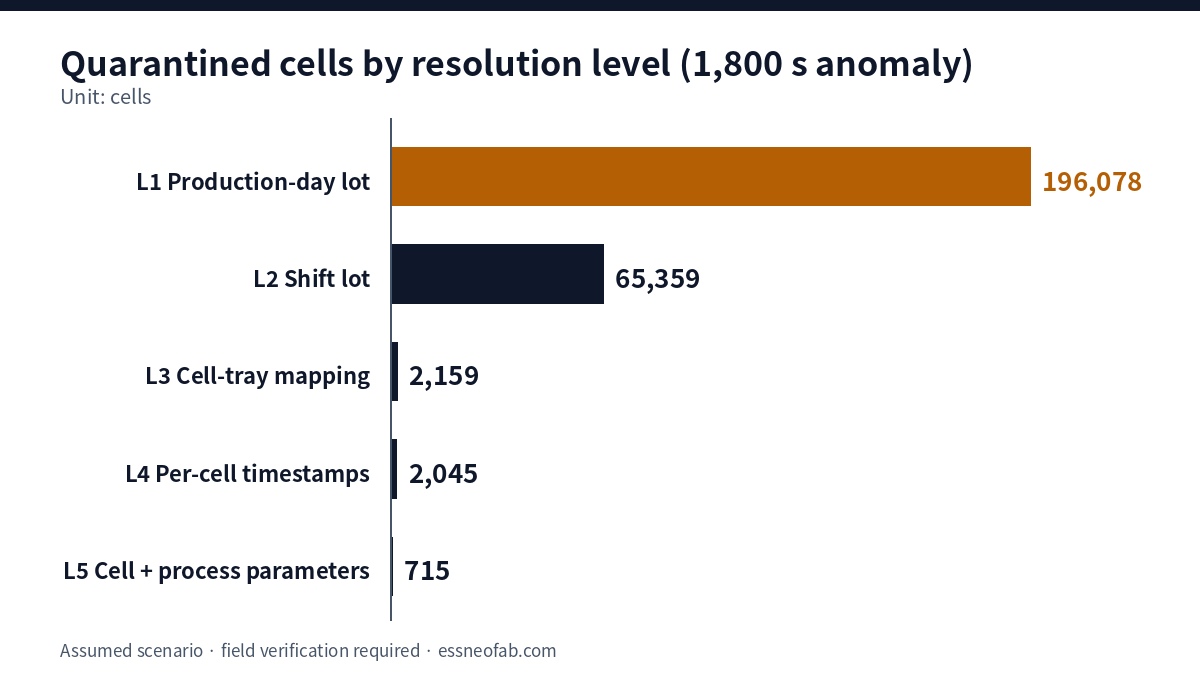
In Table 2, the L2 → L3 transition reduces 65,359 cells to 2,159 cells, about 30.3×. By contrast, L3 → L4, i.e., moving from tray-level time to cell-level time, reduces 2,159 cells to 2,045 cells, a decrease of only about 5.6%. For time-window anomalies, most of the quarantine precision is determined by time resolution, and the cell ID by itself adds little.
The roughly 2.9× reduction from L4 to L5 is different in nature. It results from selecting cells by “what value they actually received” rather than “when they passed”, and if the anomaly acted uniformly across the whole window (e.g., a sustained drift), the excursion ratio converges to 100% and the difference between L5 and L4 disappears. The value of L5 therefore depends on the distribution of anomaly types, and the excursion ratio should first be estimated from the plant’s own anomaly history.
| Level | Annual total data cost (assumed) | Savings per anomaly vs L2 | Break-even anomaly frequency | Incremental break-even vs previous level |
|---|---|---|---|---|
| L3 | KRW 50 million | about KRW 1.264 billion | 0.04 per year | — |
| L4 | KRW 150 million | about KRW 1.266 billion | 0.12 per year | about 44 per year (vs L3) |
| L5 | KRW 250 million | about KRW 1.293 billion | 0.19 per year | about 3.8 per year (vs L4) |
Table 3 shows two things. First, moving from L2 to L3 or above pays back even at an anomaly frequency of 0.04 per year (about one in 25 years). Second, incrementally, L3 → L4 needs about 44 time-window anomalies per year and is hard to justify on that basis alone, while L4 → L5 breaks even at about 3.8 per year. The case for investing in cell ID alone should be sought not in quarantine scope but in the ability to backward-trace field-returned cells and to meet customer requirements.
4. Application Limits and Difference from Existing Views
- Processes before cell ID: The electrode process precedes the creation of the cell and is therefore traced by roll and meter position. Without a link between roll-meter position and cell ID, resolution for electrode-originated anomalies drops to roll level even if downstream is at L5.
- Time alignment: The 60 s guard band at L3 assumes unsynchronised equipment PLC clocks (±30 s). L4 without time synchronisation effectively has the same quarantine scope as L3.
- Buffer mixing: The rule of adding one adjacent lot presumes buffers without guaranteed FIFO. On a line with verified FIFO, the L1 and L2 quarantine scopes shrink by about half.
This differs in nature from the question of “where the linkage breaks” addressed in Where Cell History Management Breaks at the Line Level. This article assumes the linkage is maintained and quantitatively compares quarantine scope and cost by resolution level; the effect of buffer mixing on quarantine scope should be read together with the dwell distribution in the inter-process buffer analysis.
5. Conclusions and Implications
Under the assumed scenario it is rational to prioritise resolution investment in the order “secure time resolution → link parameter values → upgrade cell ID”. Moving from lot level to time-stamped tray level alone narrows the quarantine scope by about 30×, with a break-even of about 0.04 anomalies per year. Per-cell parameter linkage narrows it a further ~2.9× when anomalies are localised, but that value must be verified against the excursion ratio in the plant’s own anomaly history.
Storage volume is not a decision variable. Storage for about 2.75 TB accumulated over 10-year retention is negligible compared with the quarantine cost of a single anomaly, and the real cost lies in time synchronisation and schema integration. This conclusion, however, depends on the assumptions of handling cost per quarantined cell and integration cost, so further verification by recalculating with the plant’s own values is required.
FAQ
Q. If the gain from cell-ID tracking is only 5.6%, does that mean cell-level tracking is over-investment?
A. No. The 5.6% is limited to forward quarantine of time-window anomalies detected in-process. When tracing backward from a single field-returned cell, without a cell ID it is impossible to identify which tray and time that cell belonged to, and the quarantine scope reverts to lot level. The cell ID should therefore be evaluated as a precondition for backward tracing.
Q. Is the handling cost of KRW 20,000 per quarantined cell too high or too low?
A. It is an assumed value and requires confirmation. Even if it is reduced to one tenth, KRW 2,000, the per-anomaly saving of L3 over L2 is about KRW 126 million, so the break-even for a KRW 50 million annual investment is still low at about 0.4 anomalies per year. The direction of the conclusion is insensitive to handling cost; only the judgement on incremental steps (L3 → L4, L4 → L5) is sensitive.
Field Application Notes
The items below can be executed first thing on Monday morning.
| Check | How to execute | Remarks |
|---|---|---|
| ☐ Determine current resolution level | Pull the record of the most recent quarantine and note which of L1–L5 in Table 1 set its scope | If levels differ by process, take the lowest as the line resolution |
| ☐ Measure equipment clock error | Collect time differences between key station PLCs and the MES server at the same instant and compute the maximum deviation (s) | The deviation sets the guard band. Target within ±1 s (assumed) |
| ☐ Recalculate recent quarantine history | Recalculate past quarantine cases with the Table 2 rules and compare with the actual number of quarantined cells | The multiple is the expected effect of resolution investment |
| ☐ Estimate excursion ratio by anomaly type | Tally the share of cells within past anomaly windows that actually exceeded control limits | Replaces the 35% assumption with plant values. If close to 100%, lower L5 priority |
| ☐ Verify electrode roll-to-cell link | Check with a sample of 10 cells whether roll ID and meter position are recorded against the cell ID at notching/stacking input | If absent, electrode-originated anomalies are quarantined at roll level |
Footnotes
[1] Traceability: A system that links the history of products, materials and process conditions through identifiers so that causes and the scope of impact can be traced.
[2] Quarantine/Containment: Holding potentially nonconforming products apart from shipment and downstream processes until disposition.
[3] Backward trace: Tracing back from a nonconforming product or anomaly signal to the causal process, time window and material. Contrasted with forward trace, which finds affected products from a cause.
[4] Takt Time: Available operating time ÷ customer-demanded quantity. Not to be confused with cycle time or FPY.
[5] Buffer: A zone holding work-in-process to absorb speed differences between processes. Without guaranteed FIFO, input and output order become mixed.
[6] Guard band: A margin added before and after the anomaly window to compensate for time and measurement uncertainty.
Sources: U.S. CPSC, “LG Energy Solution Michigan Recalls Home Energy Storage Batteries Due to Fire Hazard” (Recall No. 21-055, 2020-12-16), https://www.cpsc.gov/Recalls/2021/LG-Energy-Solution-Michigan-Recalls-Home-Energy-Storage-Batteries-Due-to-Fire-Hazard ; U.S. CPSC, same title (Recall No. 21-175, 2021-08-04), https://www.cpsc.gov/Recalls/2021/LG-Energy-Solution-Michigan-Recalls-Home-Energy-Storage-Batteries-Due-to-Fire-Hazard-0
Measurement & Calculation Conditions: Cell 100 Ah, 3.2 V; capacity 8 GWh/year (25,000,000 cells); available operating time 22,032,000 s/year; anomaly window 1,800 s; 20 stations; 24 cells per tray; time error L3 ±30 s and L4 ±1 s; one-adjacent-lot rule; L5 excursion ratio 35%; handling cost KRW 20,000 per quarantined cell; storage KRW 400,000/TB·year; and 5-year amortisation of integration cost are all assumed values. Recall quantities follow the original CPSC notices and include no judgement on cause. Results vary with the actual line’s buffer FIFO compliance and anomaly-type distribution, so field verification is required.