Inter-Process Buffers: Bigger Isn’t Always Better

Abstract — An inter-process buffer (work-in-process inventory) is not a device that gets safer as it grows. It is a range problem, bounded below by what availability demands and above by what quality tolerates. Under the assumed line conditions below, the availability-driven minimum is 2 coils while the quality-driven maximum is 1 coil — the two bounds conflict. That conflict is not resolved by enlarging or shrinking the buffer; it is resolved by reducing upstream MTTR (Mean Time To Repair) or by moving the defect-detection point ahead of the buffer. Every figure below is an assumed value set for illustration, and applying it 1:1 to a mass-production line requires separate verification.

1. The Conclusion First — Design a Buffer as a Range, Not a Size

There is no single optimal value for an inter-process buffer. The lower bound required by availability and the upper bound permitted by quality are calculated separately, and the design solution lives inside the range those two values form. If the range is empty — if the lower bound exceeds the upper bound — the problem cannot be solved by adjusting buffer size at all.

The situation is this. Equipment has been laid out to meet the takt time (available operating time ÷ customer demand quantity), and each process meets its rated line speed. The complication appears the moment an upstream process stops. With no buffer the downstream stops with it; with a buffer the downstream keeps running, but a defect originating upstream reaches downstream inspection that much later.

The question, therefore, is not “how much buffer should we hold.” It is “which is more expensive on this line — the stoppage loss or the defect propagation,” and the answer emerges only when both costs are converted into the same unit. Below they are converted into the availability term and the quality term of OEE (= Availability × Performance × Quality).

2. What a Buffer Absorbs Is Downstream Idle Time, Not Upstream Stoppage

Understanding a buffer as “it is fine if upstream stops for 1,800 s” gives you no design criterion. What a buffer actually prevents is not the upstream stoppage but the time the downstream stands with no work. The required buffer quantity is therefore the upstream stoppage duration divided by the downstream per-coil processing time.

This distinction matters because the faster the downstream runs, the more buffer is needed to survive the same stoppage. Speeding up downstream equipment raises line output but raises the buffer requirement along with it. Speed investment and buffer investment are not independent line items; they are coupled.

3. The Availability-Driven Minimum — Formula and Worked Example

The minimum buffer quantity N_min required to protect availability is derived as follows.

N_min = MTTR_upstream ÷ CT_downstream (rounded up)
MTTR_upstream : mean time to repair of the upstream process [s] · CT_downstream : downstream processing time per coil [s]

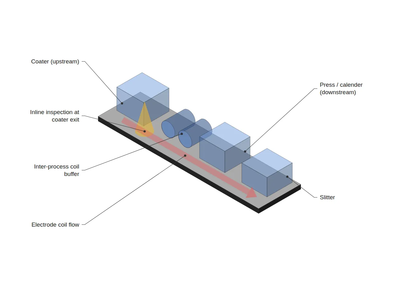
The assumed line conditions below are applied. The scope is the coater → press/calender → slitter section of the electrode process, and the buffer unit is one electrode coil.

Item	Assumed value	Converted
Coater line speed	80 m/min	1.333 m/s
Press line speed	100 m/min	1.667 m/s
Slitter line speed	120 m/min	2.000 m/s
Coil length	2,000 m	—
Coater time per coil	1,500 s	—
Press time per coil (CTdownstream)	1,200 s	—
Coater MTTR	1,800 s	—

N_min = 1,800 ÷ 1,200 = 1.5 → 2 coils. In other words, keeping the press running through a single 1,800 s coater recovery requires two coils of buffer. With only one coil, the press survives 1,200 s and then stands idle for 600 s.

4. The Quality-Driven Maximum — Propagation Scales Linearly with Buffer

A buffer delays the moment an upstream defect reaches downstream inspection. The delay equals buffer quantity × downstream per-coil processing time, and throughout that delay the upstream keeps producing under the same defect condition. The length produced before detection is the defect propagation volume.

Defect propagation volume = upstream production rate × (N × CT_downstream)

Substituting N = 2 gives a detection delay of 2,400 s and a propagation volume of 1.333 m/s × 2,400 s = 3,200 m. If the tolerated propagation volume is set at one coil (2,000 m), the upper bound becomes N_max = 2,000 ÷ (1.333 × 1,200) = 1.25 → 1 coil.

Here the lower bound of 2 coils collides with the upper bound of 1 coil. This is the point at which “bigger is better” stops holding — and equally, the point at which simply shrinking the buffer does not help either.

5. The Comparison in OEE Terms — and How to Break the Deadlock

Assume an 8-hour shift (28,800 s) containing one coater stoppage and one coater-induced defect event, and compare the two configurations. Coater output over the shift is 1.333 m/s × 28,800 s = 38,400 m.

Configuration	Availability term	Quality term	Product of the two
No buffer	(28,800 − 1,800) ÷ 28,800 = 93.75%	100%	0.938
2-coil buffer	100%	(38,400 − 3,200) ÷ 38,400 = 91.67%	0.917

Under these assumed conditions the two-coil configuration actually scores lower. This is a conditional comparison in which one stoppage and one defect each occur exactly once, so a real line must weight each event by its frequency and compare expected values. Without frequency data this table alone cannot establish that a bufferless line is superior; further verification is required.

When the range is empty, the variable to change is not the buffer but the remaining terms of the formula. First, cutting upstream MTTR to 1,200 s or below brings N_min down to 1 coil, where it meets the upper bound. Second, placing inline inspection at the coater exit moves detection ahead of the buffer, which decouples propagation volume from buffer size and removes the upper-bound constraint entirely.

Which of the two is preferable depends on capital cost and on how realistically MTTR can be shortened. The design sequence, however, is unambiguous: not fixing the buffer quantity first and fitting everything else to it, but settling MTTR and the detection point first and then choosing the buffer from whatever range remains.

FAQ

Q. Why not hold a large buffer and simply screen out defects downstream?
Downstream inspection filters defects that have already been produced; it does not undo production. Under the conditions above, a two-coil buffer presupposes 3,200 m of propagation, and that length becomes scrap or rework regardless of inspection performance. Strengthening inspection is a means of preventing escape, not of reducing occurrence.

Q. Why use MTTR rather than MTBF as the basis?
MTBF (mean time between failures) describes how often stoppages occur, whereas what a buffer must absorb is how long a single stoppage lasts. The variable that sets the lower bound on buffer quantity is MTTR; MTBF is used afterwards to check whether the buffer has room to refill. Swapping the two leads to over-sizing the buffer on a line with frequent but short stoppages.

Field Application Notes

Ordered so that it can be started on a Monday morning. Steps 1 to 3 can be completed with existing equipment logs and no additional investment.

Step	Action	Output
1	Extract the last 4 weeks of upstream stoppage events and aggregate MTTR in s	MTTR table by process
2	Measure the downstream per-coil processing time CT directly (not the rated value)	Measured CT
3	Derive the lower bound as Nmin = MTTR ÷ CT and compare with current buffer	Surplus or shortfall vs. lower bound
4	Confirm where upstream-induced defects are detected and agree a tolerated propagation volume in m	Nmax upper bound
5	If the range is empty, table either MTTR reduction or forward placement of inline inspection	Equipment improvement agenda

The “tolerated propagation volume” in step 4 is the item that quality and production must agree on as a number. If that value is never fixed, the upper bound cannot be calculated — and with no upper bound, the buffer discussion reverts to “more is safer.”

Measurement and Calculation Conditions

The line speeds, coil length, MTTR, shift duration and tolerated propagation volume in this article are all assumed values set for illustration, not measurements from any specific equipment or site. The comparison baseline is a single scenario of one upstream stoppage and one upstream-induced defect within an 8-hour (28,800 s) shift — a conditional calculation with a sample size of 1. Environmental conditions such as temperature and humidity, and equipment age, are not reflected. Applying this to a real line requires at least 4 weeks of stoppage and defect history to establish event frequencies, followed by recalculation on an expected-value basis.

Related reading — Market Trends from a Battery Process/Equipment Perspective