Cell Grading Bin Count and Grade-Specific WIP: What Module Matching History Must Retain

Abstract

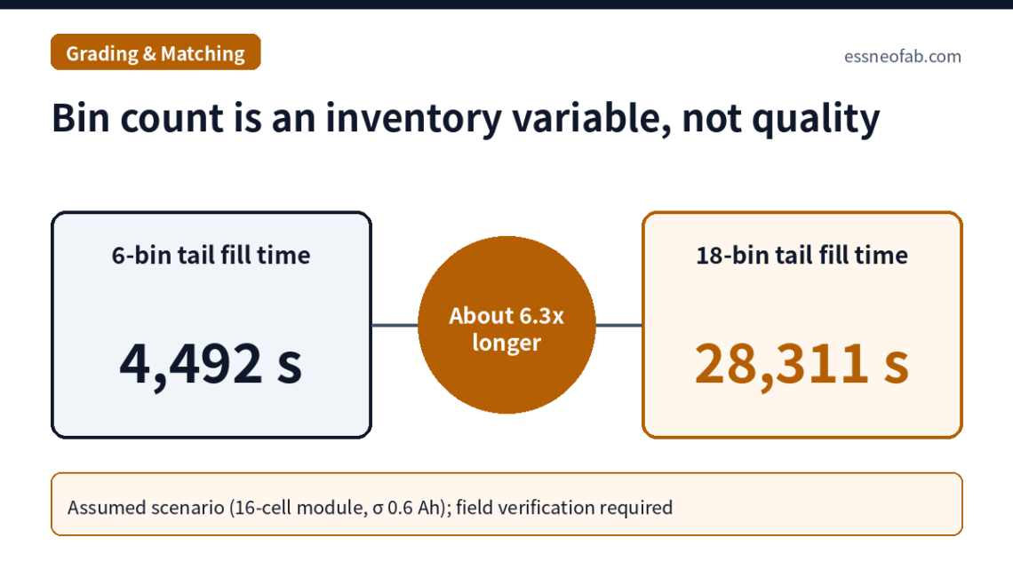
Increasing the number of cell grading bins reduces within-module capacity spread in proportion to bin width, but grade-specific waiting WIP rises in proportion to bin count, and the time for the rarest tail bin to fill one module’s worth of cells rises faster still. On an assumed line of about 4.46 million cells per year with 16-cell modules, going from 6 bins to 18 bins (6 capacity × 3 internal resistance) leaves the 0.6 Ah capacity bin width unchanged while raising average partial-fill WIP from 45 to 135 cells and tail-bin fill time from about 4,492 s to about 28,311 s.

During ramp-up (operating at 30% of rated rate) this time grows to about 94,370 s and exceeds the assumed grade validity of 86,400 s, so bin-count design is constrained not by spread but by the shelf life of the grade. For grade history to serve ESS rack imbalance analysis, what must remain is not the bin label but raw measurements, measurement conditions, bin rule version, buffer dwell time and position within the module.

1. Conclusion First — Bin Count Is an Inventory Variable, Not a Quality Variable

The number of grading^[1] bins is treated as a quality design value that reduces module spread, but on the line it acts first as an inventory design value that determines grade-specific WIP^[2] and waiting time. And when that waiting time grows long, the grade itself becomes stale.

Situation (S): Cells that have completed formation and aging are graded by measured values such as capacity, internal resistance^[3] and OCV, and the module assembly process matches^[4] only cells of the same grade or within tolerance. Complication (C): The finer the bins become to reduce spread, the lower the inflow rate into each bin, and cells stay in grade-specific buffers until one module’s worth is accumulated. Question (Q): How much do bin count and matching tolerance move grade-specific WIP and module spread, and in what form must that history remain for field use? Answer (A): WIP rises linearly with bin count, and tail-bin waiting time rises superlinearly. What field analysis needs is not the bin label but the raw measurements and rules that produced it.

This article does not address the internal-chemistry causes of cell spread. Taking the existence of spread as given, it analyzes only the line buffers and data structures that classify, hold and trace that spread.

2. Mechanism — Bins Create Buffers, and Buffers Make Grades Stale

When a module consists of M cells, the occupancy probability of bin i is p_i and the cell inflow rate is λ, the time for bin i to fill one module’s worth is M ÷ (λ · p_i). Because each bin always holds 0 to (M−1) partially accumulated cells, steady-state average partial-fill WIP is approximated as N × (M−1) ÷ 2 and the maximum as N × (M−1). Average WIP is therefore linear in bin count N, but waiting time is dominated by the smallest p_i.

The occupancy probability of tail bins at both ends of the distribution falls sharply as bins are subdivided. Applying two-dimensional classification (capacity × internal resistance) makes the tail-bin probability the product of the two axes’ probabilities, shrinking it by an order of magnitude or more. Because OCV changes during a long wait, the grade assigned at classification no longer represents the cell’s state at assembly.

History item to retain	Recording unit	Problem in rack imbalance analysis if missing
Raw measurements (capacity, internal resistance, OCV)	Values per cell ID	With only a bin label, differences within the bin width (e.g., 0.6 Ah) cannot be recovered
Measurement conditions (temperature °C, measurement time)	Per measurement event	Whether temperature correction was applied is unknown, so lot-to-lot comparison lacks controlled variables
Bin rule version[5]	Per classification event	The same label “B2” means different ranges at different times, making label comparison meaningless
Buffer entry and exit times	Per cell ID	The relationship between dwell time and OCV change cannot be separated
Module ID + position in module, rack ID + position in rack	Per assembly event	Cell voltage channels reported by the BMS[6] cannot be mapped back to manufacturing history

The baseline in Table 1 is storing bin labels only. Under this approach, even when cell voltage spread is observed at the rack, it cannot be determined whether the cause is manufacturing spread, buffer dwell or position within the module (thermal environment). The implication is that a grade label is an output of analysis, not source data; retaining only labels means field analysis starts after the source data have been lost.

3. Assumed Scenario — Grade-Specific WIP by Bin Count

The assumptions are as follows. With about 4,464,286 cells per year (4 GWh/year ÷ 280 Ah, 3.2 V) and available operating time of 28,512,000 s, takt time^[7] is about 6.39 s per cell and cell inflow rate λ is about 0.157 cells/s. Modules have 16 cells (1P16S), capacity follows a normal distribution with a standard deviation of 0.6 Ah, and bins divide the ±3σ range into equal widths, with values outside the range assigned to the end bins.

Bin configuration	Capacity bin width	Minimum bin occupancy probability	Average partial-fill WIP	Maximum partial-fill WIP	Tail-bin fill time
3 bins (capacity)	1.2 Ah	15.9%	22.5 cells	45 cells	about 644 s
6 bins (capacity)	0.6 Ah	2.28%	45 cells	90 cells	about 4,492 s
9 bins (capacity)	0.4 Ah	0.98%	67.5 cells	135 cells	about 10,411 s
12 bins (capacity)	0.3 Ah	0.62%	90 cells	180 cells	about 16,456 s
18 bins (6 capacity × 3 internal resistance)	0.6 Ah	0.36%	135 cells	270 cells	about 28,311 s

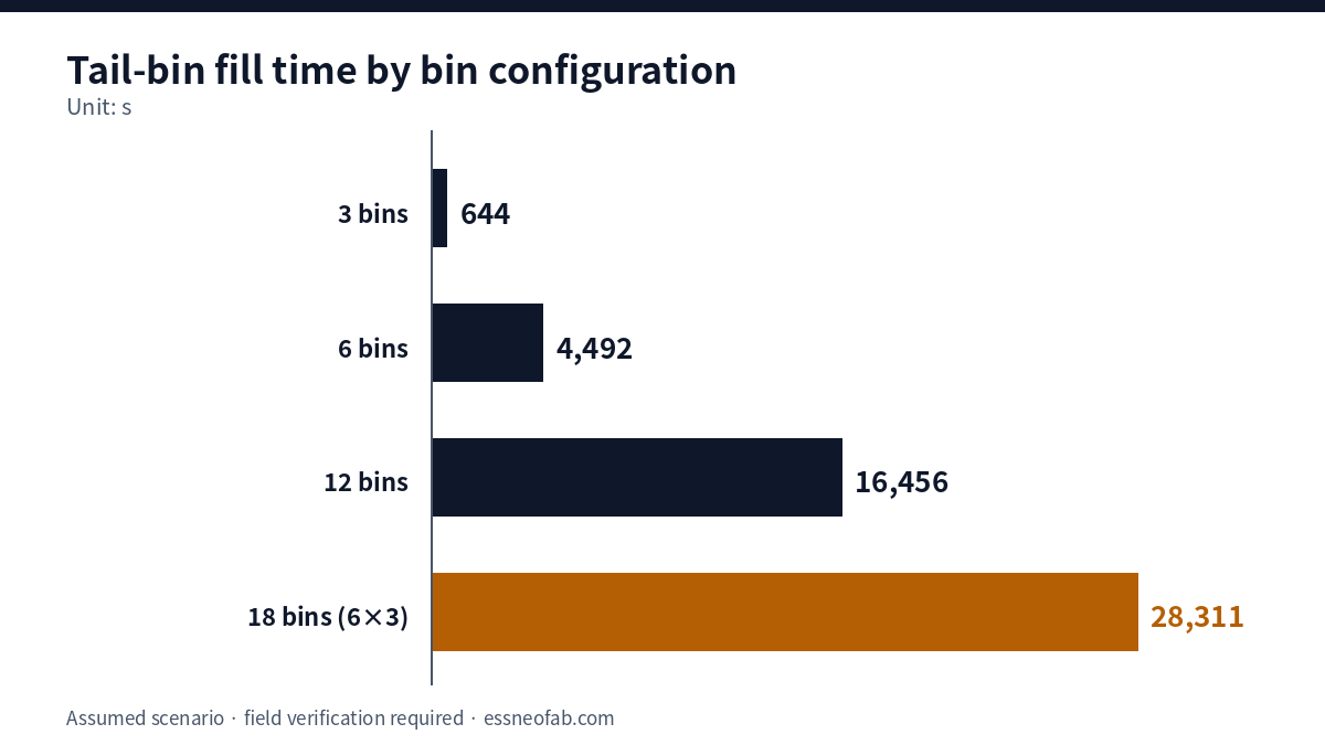
Taking 6 bins as the baseline in Table 2, 12 bins halve the upper bound of within-module capacity spread from 0.6 Ah to 0.3 Ah at the cost of doubling average WIP (45→90 cells) and increasing tail-bin fill time about 3.7-fold (4,492→16,456 s). Two-dimensional classification with 18 bins leaves the capacity bin width unchanged while increasing tail-bin fill time about 6.3-fold. The implication is that the cost of bin subdivision appears first in tail-bin waiting time, not in average WIP.

This time is inversely proportional to production rate. When operating at 30% of rated rate during ramp-up, the tail-bin fill time of the 18-bin configuration becomes about 94,370 s, exceeding grade validity if that validity is assumed to be 86,400 s. Tail-bin cells must then be re-measured or mixed with adjacent bins before module insertion, and in either case the handling history itself must be recorded as well.

4. Tolerance Matching and Limits of Application

The alternative to binning is tolerance matching. Instead of fixed bins, selecting from the buffered cells a combination whose within-module spread falls within tolerance allows cells near bin boundaries to be grouped together, reducing tail-bin dwell. In this case, however, cells carry not even a bin label, so post-hoc reproduction is impossible unless the matching algorithm version and tolerance settings are recorded per assembly event.

This analysis differs from Inter-Process Buffers, which addresses buffer capacity in general. Whereas that article deals with buffers that absorb differences in equipment uptime, the buffer here is a “grade-dispersed WIP” created by classification rules alone, regardless of uptime differences. Rack-level documentation requirements also connect to the scope of NFPA 855 2026 Edition, ESS Rack Design and Traceability Documents, but whether the Table 1 items are requirements of that standard needs separate review.

As limits of application, the assumptions of a normal distribution, equal-width bins and a single lot do not reflect real distribution asymmetry or lot changeovers. If bins are operated separately per lot, WIP multiplies by the number of lots open at once. The EU Battery Regulation (2023/1542) battery passport applies from 18 February 2027 to industrial batteries above 2 kWh and others, but whether it must include cell grade history requires confirmation.

5. Conclusions and Implications

Bin count and matching tolerance are line variables that jointly determine not only module spread but also grade-specific WIP, tail-bin waiting time and the shelf life of the grade. In the assumed scenario, doubling bin count doubled average WIP but increased tail-bin waiting time about 3.7-fold, and during ramp-up a range emerged that exceeds grade validity.

Bin count must therefore be verified at the lowest operating rate, not at the rated rate. And grade history becomes a basis for tracing rack imbalance in the field back to the manufacturing stage only when raw measurements, measurement conditions, bin rule version, buffer dwell time and position within module and rack are retained as one bundle. The contribution of module spread to rack imbalance, however, varies with operating conditions, so further verification is required.

FAQ

Q. Since finer bins reduce module spread, doesn’t field imbalance also fall in the end?
A. Looking only at spread at the time of manufacture, yes. But tail-bin cells stay longer in the buffer and enter modules with OCV having changed in the meantime. Subdivision thus reduces classification-time spread while bringing a new variable, dwell-time spread, into the module. Which effect is larger can be determined with statistical significance only if buffer dwell time has been recorded.

Q. Since the BMS performs cell balancing, isn’t manufacturing grade history unnecessary in the field?
A. Balancing corrects voltage spread during operation but does not reveal its cause. When balancing load on a specific rack is significantly higher, manufacturing history is needed to distinguish whether the cause is the manufacturing lot, tail-bin dwell or installation position, and this judgment must be combined with operating data that require separate review.

Field Application Notes

The following items can be executed on Monday morning.

Check	How to execute	Remarks
☐ Calculate occupancy probability per bin	Count cells per bin from recent lots’ grading results and identify the bin with minimum occupancy probability	Calculate tail-bin fill time M ÷ (λ · p) from that probability
☐ Identify the longest-dwelling cells in the buffer	Query entry times in the grade buffer and check the bins of the top 20 cells by dwell time	If entry time is not recorded, that is the first improvement item
☐ Document a grade validity criterion	Specify within how many s after classification a cell must be inserted into a module, and whether to re-measure or mix with an adjacent bin when exceeded	86,400 s assumed in this article; confirm your own criterion
☐ Add a bin rule version field	Store the version ID of the bin boundary set per classification event in the MES grade table	Tag historical data retroactively by effective period
☐ Recalculate at ramp-up rate	Using the Table 2 method, recalculate tail-bin fill time at 30% of rated rate	If any bin exceeds validity, consider fewer bins during ramp-up

---

Footnotes
[1] Grading: The process step that classifies cells into grades according to reference ranges for measured values (capacity, internal resistance, OCV, etc.).
[2] WIP (Work In Process): Intermediate inventory waiting for the next operation between processes. In this article, the number of cells waiting in grade-specific buffers.
[3] Internal Resistance (IR): The resistance component measured between cell terminals. Treated in this article only as a classification input.
[4] Matching: Selecting and grouping cells so that cell-to-cell spread within a module stays within tolerance.
[5] Bin Rule Version: An identifier assigned to a set of bin boundary values. It prevents the same grade label from meaning different ranges at different times.
[6] BMS (Battery Management System): The control layer that monitors cell and module voltage and temperature and performs protection and balancing.
[7] Takt Time: Available operating time ÷ customer demand quantity. Not to be confused with Cycle Time or FPY.

Sources: Bizhong Xia et al., “Using Self Organizing Maps to Achieve Lithium-Ion Battery Cells Multi-Parameter Sorting Based on Principle Components Analysis”, Energies 12(15), 2019, https://www.mdpi.com/1996-1073/12/15/2980 (single-parameter sorting ignores relationships among parameters; multi-parameter sorting improved module SOC consistency). Regulation (EU) 2023/1542, EUR-Lex, https://eur-lex.europa.eu/eli/reg/2023/1542/oj/eng. “Battery passport”, Wikipedia, https://en.wikipedia.org/wiki/Battery_passport (applies from 2027-02-18 to LMT, industrial above 2 kWh and EV batteries). “Article 77 Battery Passport”, TracePass, https://www.tracepass.eu/regulatory/battery-articles/article-77.

Measurement & Calculation Conditions: Line capacity of 4 GWh/year, 280 Ah, 3.2 V cells (about 4,464,286 cells per year), available operating time of 28,512,000 s, takt time of about 6.39 s, 16-cell modules (1P16S), normally distributed capacity with a standard deviation of 0.6 Ah, equal-width bins over ±3σ, 3 internal-resistance bins, a single lot, grade validity of 86,400 s and a ramp-up operating rate of 30% are all assumed values. Results vary with actual distribution shape, lot changeovers and buffer operating rules, so field verification is required, and pilot-condition results are not applied 1:1 to mass-production lines.