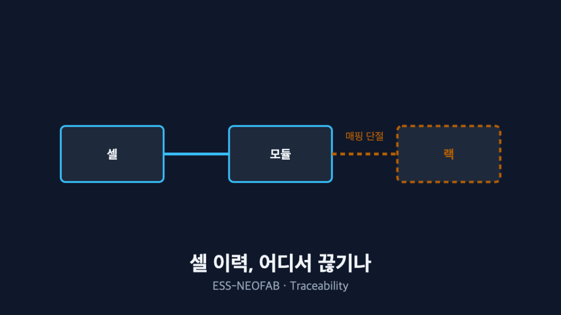
Cell Traceability: Where Does It Break Down at the Line Level?

Abstract — The value of traceability is measured by one thing only: how far it narrows the recall scope when a defect appears. What matters is not the precision of cell-level data but whether the mapping survives each process boundary — and when one mapping link breaks, the recall scope does not grow by addition but is multiplied by that level’s capacity. Under the assumed site configuration below, a missing module-to-rack-slot mapping widens the suspect population from 24 cells to 480, a factor of 20. Every figure below is an assumed value for illustration and must be recalculated against an actual site configuration.

1. The Conclusion First — The Cost of a Broken Link Scales Multiplicatively

Traceability investment is usually framed as “how precise should the tracking be.” But when a defect actually occurs, the variable that sets the cost is not precision — it is the first mapping level that breaks. Everything below that level exists as data but cannot be reconstructed.

The situation: at cell receiving, cell-level history is secured by QR or barcode. The complication is that as assembly proceeds, only the higher-level identifier gets recorded and the correspondence to the lower level is dropped. The question is “which boundary do we close first,” and the answer falls out of multiplying each boundary’s capacity to get the recall scope.

2. History Breaks at Process Boundaries

Process boundary	Common cause of the break	Information that becomes unrecoverable
Cell receiving → module assembly	Missed barcode scan, switch to manual entry	Cell lot to module correspondence
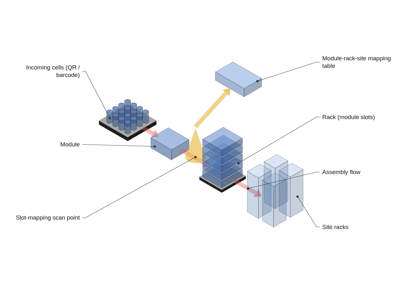
Module → rack assembly	Module ID to rack slot mapping not recorded	Which module went into which slot
Rack → system commissioning	BMS parameter change history not recorded	Which parameters governed initial cycling

The most common pattern is that cell-level QR codes are scanned all the way through module assembly, and then — the moment the module enters a rack — only the rack number is recorded and the slot is omitted. Once that link breaks, a single defective module puts the entire rack under suspicion.

3. Calculating Recall Scope — Where the Break Sits Sets the Multiplier

The recall scope for a single defective cell is calculated below against an assumed site configuration. The configuration is a value set for illustration.

24 cells per module · 20 modules per rack · 40 racks per site → 19,200 cells per site

Where history breaks	Smallest recoverable unit	Cells recalled	vs. full traceability
Nowhere (full cell-level tracking)	Cell	1	1×
Cell → module mapping missing	Module	24	24×
Module → rack slot mapping missing	Rack	480	480×
Rack → site mapping missing	Site	19,200	19,200×

The point worth noting is that the growth is not linear. A single missing module-to-slot mapping takes the recall scope from 24 cells to 480 — a factor of 20. Since modules per rack is itself the multiplier, a design change that raises rack density raises the loss from a broken link by exactly the same ratio.

This calculation assumes the defect originated in a single cell. If the root cause is a material deviation spanning an entire lot, the recall scope is set by the lot regardless of mapping, so these multipliers cannot be asserted to apply to every defect type.

4. The Takt-Time Cost of Adding a Scan Point

Closing a mapping gap means adding a scan point at the process boundary, and scanning consumes takt time (available operating time ÷ customer demand quantity). Assume slot mapping is scanned for 20 modules during rack assembly.

Item	Assumed value
Scan time per module	2 s
Modules per rack	20
Added time per rack	40 s
Rack assembly takt time	600 s
Share of takt time	6.7%

If takt-time headroom exceeds 6.7%, the scan can be absorbed without adding equipment; if not, the scan must be run in parallel with assembly or converted to automatic reading. The basis for the investment decision is putting two numbers — “recall scope 480 cells → 24 cells” and “6.7% of takt time” — on the same table and comparing them.

5. Design Principles — Continuity Before Precision

Three principles follow from a line-level view. First, place an automatic scan point at every process boundary and minimize manual-entry segments. Manual segments defeat later reconstruction not because of their omission rate but because of the randomness of the omissions.

Second, maintain the module-rack-site three-level mapping as a separate table. A rack number alone cannot reconstruct its contents, so a higher-level record must never be treated as a substitute for the lower-level mapping. Third, log BMS parameter changes separately, because identical cells follow different degradation paths when their initial cycling conditions differ.

FAQ

Q. Does traceability have to be designed perfectly from the start?
No. As the table shows, only one boundary opens the multiplier the widest, and closing that boundary alone removes most of the recall scope. Automating one or two bottleneck boundaries first yields more return than applying the full scheme across every process at once.

Q. We already have an MES — is a separate mapping table really necessary?
Having an MES and having mapping continuity are separate questions. If the MES is configured to collect rack-level production results only, the system exists but the slot mapping does not. What has to be checked is not the presence of an MES but the granularity of the events it collects, and that can only be established by opening the current event list and reading it.

Field Application Notes

Step	Action	Output
1	List the events the MES currently collects, grouped by process boundary	Event list per boundary
2	Flag boundaries where the lower-level ID is not recorded alongside the higher-level one	List of broken boundaries
3	Multiply each boundary’s capacity to derive the recall-scope multiplier	Multiplier table by boundary
4	Measure scan time at the single largest-multiplier boundary and compute its share of takt time	Takt-time impact figure
5	Put recall-scope reduction and takt-time share on one table and table the investment	Scan-point addition agenda

Steps 1 to 3 can be completed with the existing MES configuration screens and the line layout sheet, with no new investment. The scan time in step 4 must be measured from actual operator motion rather than taken from a rated value, and it varies considerably with operator experience.

Measurement and Calculation Conditions

24 cells per module, 20 modules per rack, 40 racks per site, a 2 s scan and a 600 s rack assembly takt time are all assumed values set for illustration, not measurements from any specific site. The recall-scope calculation assumes the defect originates in a single cell and that the entire smallest recoverable unit containing that cell is recalled; it does not apply to lot-level material defects or process-condition excursions. It is a single scenario with a sample size of 1, and real application requires obtaining the incidence rate by defect type from recent quality history and recalculating on a weighted-average basis.

Related reading — BMS, PCS, EMS: Why Do the Three ESS System Layers Run at Different Speeds?