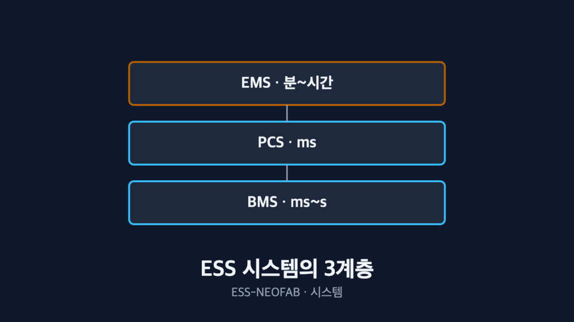
BMS, PCS, EMS: Why Do the Three ESS System Layers Move at Different Speeds?

Abstract — Describing an ESS as “a battery with a PCS attached” is only half right. BMS, PCS and EMS each make decisions on a different time axis, and the gap between their control periods is not a qualitative remark but a quantitative one of roughly seven orders of magnitude (10⁷). That gap is why the three layers cannot be collapsed into one control loop, and whether a protection response can ride on the communication chain must be judged by the product of chain latency and voltage rise rate. Every figure below is an assumed value for illustration and must be recalculated against actual equipment specifications.

1. The Conclusion First — The Three Layers Are to Be Separated, Not Merged

System integration discussions often drift toward “let’s consolidate the control.” But the three ESS layers watch different physical phenomena, and those phenomena have different time constants to begin with. What needs to be unified is not the control loop but the matching conditions of the interfaces between layers.

The situation is the point just after rack assembly and before system commissioning. The complication is that the three layers come from different vendors and different firmware generations. The question is “which decision belongs to which layer,” and the answer emerges as soon as the permissible latency of each decision is written down.

2. The Three Layers See Time Seven Orders of Magnitude Apart

Layer	Representative control period (assumed)	Primary decisions	Phenomenon monitored
PCS	0.1 ms (10 kHz)	DC-AC conversion, current control	Switching period, current ripple
BMS	10 ms	Cell voltage and temperature protection, balancing	Cell voltage rise, temperature rise
EMS	900 s	Charge/discharge scheduling, grid dispatch	Tariff periods, demand forecast

The PCS at 0.1 ms and the EMS at 900 s differ by a factor of 9,000,000. Put that spread inside one control loop and the fast side is pinned to the slow side’s period while the slow side cannot carry the fast side’s computational load. Layer separation is not a design convenience; it is a structure the time constants impose.

The practical implication is this. Before moving a decision up to a higher layer, confirm that the decision’s permissible latency exceeds that layer’s control period. Skip that check and push a safety-related decision up to the EMS, and the phenomenon is over before the instruction arrives.

3. Can Protection Ride on the Communication Chain? — The Decision Rule

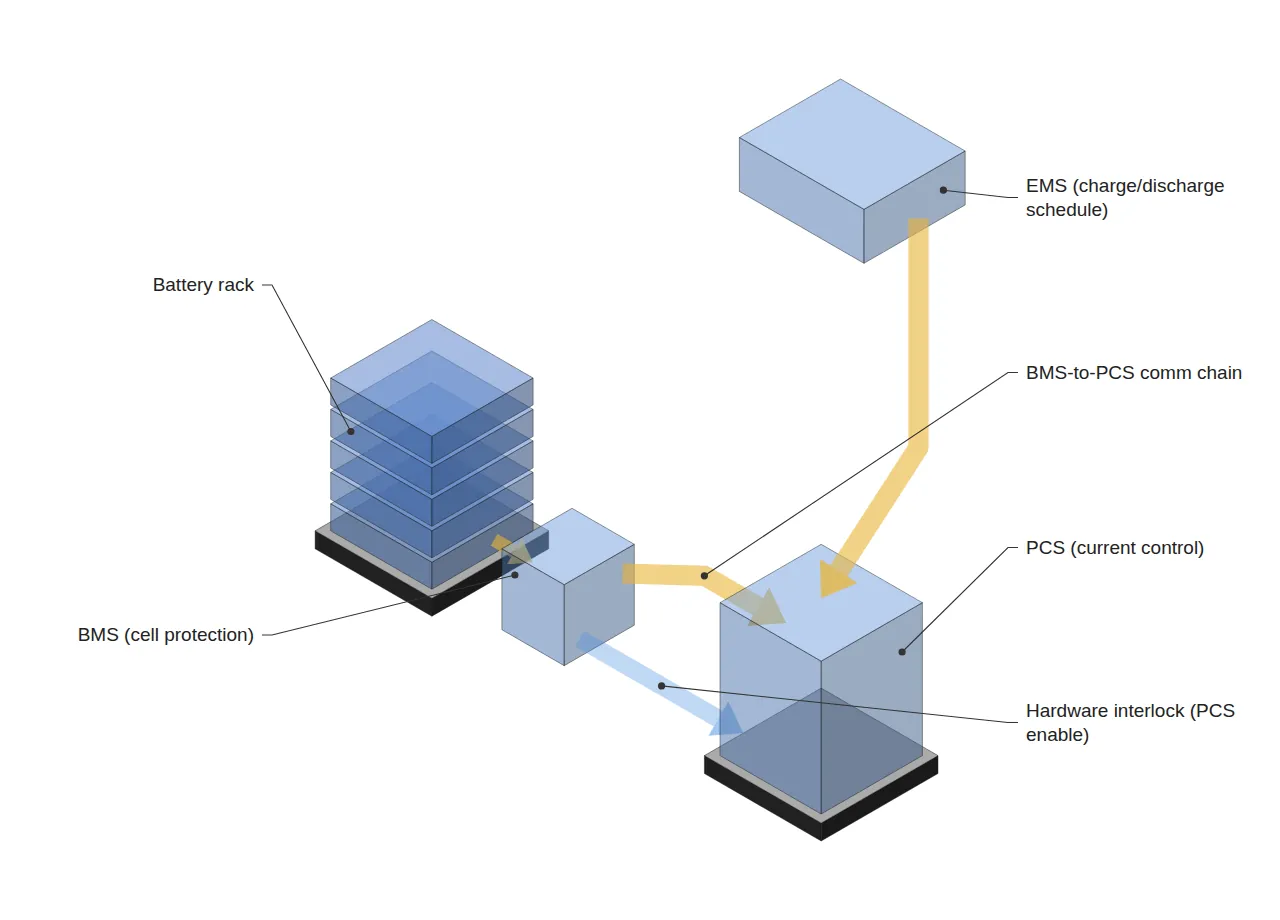
If cell overvoltage protection is built as BMS detection → communication → PCS current cutoff, the question is how much further the cell voltage rises during the total chain latency.

Overshoot = voltage rise rate × total chain latency

Segment	Assumed latency
BMS overvoltage detection period	10 ms
BMS → PCS communication transfer	20 ms
PCS command execution	30 ms
Total chain latency	60 ms

Charging condition	Voltage rise rate (assumed)	Overshoot over 60 ms	vs. 0.05 V allowance
Rated current	0.5 V/s	0.030 V	Within
Twice rated	1.0 V/s	0.060 V	Exceeded

Under rated conditions the communication chain is adequate for protection, but the moment current doubles the same chain exceeds the allowed overshoot. In other words, whether an interlock is required is a function of operating condition, not of equipment specification, and the judgment must be made at maximum current.

When it is exceeded, the response is not to make the communication faster but to take the protection decision off the communication path entirely. A hardware interlock in which a BMS output contact directly breaks the PCS enable signal is the standard solution. These are assumed figures, however, so the rise rate a given line actually exhibits must be established by measurement.

4. Where It Binds at the Line Level — The Layers Are Not Ready Together

On a production line, the three layers cause trouble not through performance but through readiness timing. Rack assembly may be complete, but if the BMS firmware version does not match the protocol the EMS expects, a communication timeout appears at commissioning.

A representative line issue is mixing two lots from different cell manufacturers into one rack. When BMS balancing reference values differ by lot, initial SOC spread widens and balancing during commissioning takes longer than planned. This surfaces as a process-planning problem rather than a quality problem, and it is prevented by keeping lots separated at rack level.

5. Separate the Maintenance Windows by Layer

When an EMS schedule change overlaps a BMS balancing cycle, balancing is interrupted or restarted and cell-to-cell spread fails to converge. The two operations sit on different time axes, so there is no reason to place them in the same window — and separating them costs nothing.

The design sequence for the three layers follows. Write down the permissible latency of each decision, place each decision in the lowest layer that satisfies that latency, and move to hardware only what cannot ride on the communication chain.

FAQ

Q. Does standardizing on one vendor for BMS and PCS solve this?
Only partly. Even with the same vendor, different rack generations frequently diverge in protocol version. More importantly, a single vendor does not eliminate the latency of the communication chain itself. The judgment in section 3 must be performed regardless of vendor composition.

Q. Wouldn’t a faster communication link remove the need for a hardware interlock?
Of the 60 ms total chain latency, communication transfer accounts for 20 ms — so even reducing transfer to zero leaves 40 ms. At the 1.0 V/s rise rate of the twice-rated case, 40 ms gives 0.040 V, inside the 0.05 V allowance, but with only 0.010 V of margin. As long as the detection period and command execution time remain, faster communication buys limited headroom, and that headroom is weak grounds for a design margin.

Field Application Notes

Step	Action	Output
1	List every decision the system makes and write each one’s permissible latency in ms or s	Decision-latency table
2	Extract BMS detection period, communication transfer and PCS execution time from datasheets and total the chain latency	Chain latency value
3	Measure cell voltage rise rate at maximum current and compute the overshoot	Overshoot vs. allowance
4	Classify only the decisions that exceed the allowance as hardware interlock candidates	Interlock candidate list
5	Record BMS firmware version per rack by lot and pre-check before EMS integration	Firmware cross-reference
6	Separate the EMS schedule-change window from the BMS balancing window in the maintenance plan	Separated maintenance windows

Steps 1 and 2 are possible from datasheets alone; only step 3 requires measurement. The firmware cross-check in step 5 costs nothing if done at rack receiving, but requires reopening racks if the mismatch is found at commissioning.

Measurement and Calculation Conditions

Control periods of 0.1 ms / 10 ms / 900 s, chain latencies of 10 + 20 + 30 ms, voltage rise rates of 0.5 and 1.0 V/s and a 0.05 V allowed overshoot are all assumed values set for illustration, not the specification of any product. Voltage rise rate varies with charging current, SOC region and cell temperature, and the article uses a linear approximation for a single condition. Actual judgments must use a measured rise rate at maximum charging current, high SOC and low temperature (below 0 °C); concluding from a sample size of 1 that no interlock is needed would not be appropriate.

Related reading — Between the Battery Rack and the PCS: Two Points Where the Interface Diverges