A 2.5 GWh Line Fed Only 1 GWh of Cells — OEE of 36.9% and 83.8% Describe the Same Line

Abstract

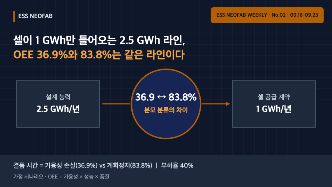
On 18 September 2026, India’s Advait Group signed a master supply agreement with Hithium for 314 Ah LFP prismatic cells. The agreement covers up to 1 GWh over the next year, while the cell-to-container assembly plant that will use these cells is being built for 2.5 GWh per year. On a line whose cell supply is 40% of design capacity, how OEE¹ is calculated changes operating decisions. Under an assumed scenario, the same line with the same output can be reported at an OEE of 36.9% or of 83.8%. The difference comes not from the equipment but from the classification rule for the OEE denominator — whether cell-shortage time is removed as planned downtime or counted as availability loss.

1. Conclusion First — On a Supply-Constrained Line, the Denominator Rule Decides OEE

Under the assumed conditions, recording cell-shortage time as availability loss yields an OEE of 36.9%; separating shortage time as planned downtime and matching available operating time to supply yields 83.8%. The 46.9-point gap comes entirely from the cell-supply constraint, and not a single point of it can be recovered through equipment improvement.

Situation (S): BESS assembly plants often source cells externally, and early in a ramp-up there is a period in which contracted cell volume is smaller than assembly capacity. Complication (C): If the line runs at design speed in this period, it stops for lack of cells, and the indicator swings widely depending on how that time enters OEE. Question (Q): What should OEE and takt time² be based on in this case? Answer (A): Redefine available operating time to match cell supply, and separate shortage time as planned downtime. Only then does OEE point to equipment performance.

The assumption this article challenges is the reading that “low OEE means an equipment problem.” On a supply-constrained line, the reason for low OEE may lie outside the equipment, and improvement activity then heads in the wrong direction.

2. Announced Facts and Assumed Conditions

The disclosed facts are as follows. Advait Battery Ecosystem (part of Advait Energy Transitions) signed a master supply agreement (MSA) with Hithium for LFP prismatic cells. Hithium will supply 314 Ah LFP prismatic cells, and the agreement provides for offtake of up to 1 GWh over the next year. Advait’s 2.5 GWh/yr cell-to-container assembly plant is under construction in Gangad, Gujarat, and covers module and pack assembly, container integration and system commissioning. EMS and PLC/SCADA design are being carried out in collaboration with Adaptive Engineering. The start of commercial production is described only as “soon”; no date is confirmed.

Available operating time, design cycle time and intrinsic equipment loss rates have not been disclosed. All figures below are assumptions that require measured verification.

Item	Value	Basis
Energy per cell	1.0048 kWh	314 Ah × 3.2 V (nominal voltage assumed)
Cells at design capacity	2,488,057 per year	2.5 GWh ÷ 1.0048 kWh
Cells at contracted supply	995,223 per year	1 GWh ÷ 1.0048 kWh
Annual available operating time (nominal)	6,000 h = 21,600,000 s	Assumption
Design cycle time (per cell input)	8.0 s/cell	Assumption
Intrinsic A · P · Q	90% · 95% · 98%	Assumption (intrinsic OEE 83.8%)

On nominal available operating time, takt time is 8.68 s/cell for 2.5 GWh of demand and 21.70 s/cell for 1 GWh. The design cycle time of 8.0 s leaves about 8% margin against the 2.5 GWh takt time.

3. Mechanism — Same Output, Three Ways of Recording

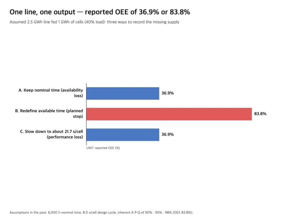
The same year of assembling 995,223 cells is recorded in three ways. OEE = availability × performance × quality, and good output is identical in all three cases.

Method	Operation	Treatment of shortage time	Reported OEE	Where the loss is recorded
A. Keep nominal time	Schedule 6,000 h, run at design speed, stop when no cells	Availability loss	36.9%	Availability
B. Redefine available operating time	Schedule only about 2,639 h to match supply	Planned downtime (excluded from denominator)	83.8%	Intrinsic equipment losses only
C. Run slower	Schedule 6,000 h, stretch cycle to about 21.7 s	Performance loss	36.9%	Performance

Method A’s OEE is (995,223 × 8.0 s) ÷ 21,600,000 s = 36.9%. In Method C the same loss merely moves from availability to performance; the value is the same. Method B sets the required planned time at 995,223 × 8.0 ÷ 0.838 ≈ 9,502,069 s (about 2,639 h), so the only remaining OEE losses are intrinsic equipment losses. Takt time then becomes 2,639 h ÷ 995,223 cells ≈ 9.55 s/cell.

Prior art (US7698011B2) likewise defines load time as ‘possible operating time minus planned equipment downtime’ and calculates OEE on that basis. Whether time in which there is no plan to use the equipment because of supply constraints is placed in this planned downtime is the classification rule that separates Methods A and B.

4. Line-Level Implications — Which Method to Choose

None of the three methods is a wrong calculation. The issue is the decisions made by looking at the indicator.

• If Method A or C is reported as is, the improvement organisation will try to raise availability (A) or performance (C). But the 46.9 points between 36.9% and 83.8% are a loss caused by the absence of cells, and cannot be recovered through equipment maintenance or speed improvement.
• If Method B is reported, OEE accurately reflects equipment condition, and the supply constraint appears in a separate indicator (loading ratio of 40% against design capacity). Staffing and shift patterns can also be planned on a 2,639 h basis.

In practice, it is reasonable to use Method B as the default while reporting the loading ratio (supply ÷ design capacity) alongside OEE. If OEE stays at 83.8% while the loading ratio rises from 40% to 100% during ramp-up, the equipment is fine; if OEE falls, that is where equipment improvement begins.

Method C (running slower) is a common choice on assembly lines, but whether slowing down affects process quality (e.g., fastening or welding conditions) needs separate confirmation, because changing speed can move validated process conditions.

5. Limitations and Scope

This calculation assumes cell supply arrives evenly through the year and that parts other than cells (racks, containers, PCS, etc.) are unconstrained. In reality, cell receipts arrive in lots, so shortage and surplus alternate and the Method B schedule may need monthly readjustment. In addition, “up to 1 GWh” is a ceiling; if actual offtake is smaller, the loading ratio falls below 40%.

The conclusion of this article is limited to supply-constrained periods. On a line with a loading ratio close to 100%, the difference between the three methods disappears and OEE again becomes a direct indicator for equipment improvement. All figures are a calculation scenario and require further verification before application to a production line.

FAQ

Q. Isn’t removing shortage time as planned downtime just a trick to make OEE look better?

Not if the loading ratio is always reported alongside it. On the contrary, putting shortages into availability loss mixes equipment breakdowns and supply shortfalls in one bucket and makes root-cause analysis impossible. The key is not ‘whether to remove it’ but ‘which indicator exposes it separately’.

Q. If takt time changes to 9.55 s, does the 8.0 s design cycle time lose its meaning?

No. 8.0 s is the equipment’s capability (cycle time), and 9.55 s is the takt time calculated from demand conditions. The two values have different definitions and are not to be used interchangeably. Method B runs at the 8.0 s speed but shortens scheduled time to match takt.

Field Application Notes

Check	How to execute	Remarks
☐ Separate ‘material shortage (external supply)’ in stop codes	Distinguish equipment breakdown, setup and material-shortage codes, and subdivide shortages by supply cause	The classification rule determines how OEE is read
☐ Create a loading-ratio indicator	Calculate confirmed supply ÷ design capacity monthly and report it next to OEE	40% in this assumed case
☐ Recalculate available operating time	Compute required scheduled time as confirmed supply × design cycle time ÷ intrinsic OEE	Basis for shift and staffing plans
☐ Check process-condition impact before running slower	Before changing speed, confirm the validated range of fastening, welding and inspection conditions	If outside the validated range, prefer Method B
☐ Agree on criteria for judging OEE trends during ramp-up	Judge equipment abnormality by whether OEE holds its intrinsic value while the loading ratio rises	Baseline: Method B value

---

Footnotes
¹ OEE (Overall Equipment Effectiveness): Availability × performance × quality. Not to be confused with cycle time or FPY.
² Takt Time: Available operating time ÷ customer demand. Here, confirmed supply is treated as the effective demand.

Sources: pv magazine India, “Advait Group signs 1 GWh LFP cell supply agreement with Hithium” (2026-09-18). ESS News article of the same title (2026-09-18). Prior-art reference patent (no new patents were found in the most recent 7 days, so the search was extended to 30 days; no newly published items were confirmed in that window either, so the patent is cited as general prior art only): US7698011B2 (Operating condition monitoring apparatus, method for monitoring operating condition and program, Omron, published 2010-04-13).

Measurement and calculation conditions: Nominal cell voltage 3.2 V, annual available operating time 6,000 h, design cycle time 8.0 s/cell, intrinsic A·P·Q of 90%·95%·98% and even annual cell supply are all assumptions. The comparison baseline is Method B in Table 2. Temperature, humidity, sample size and similar measurement conditions are not applicable (calculation scenario). Not to be cited for finalising operating indicators without measured verification.

---

Other Articles in This Issue

ESS NEOFAB WEEKLY No.02 · Research window 2026-09-16 to 2026-09-23

• 45 Days from Pohang to Georgia — Safety Stock at an Intercontinental Cathode Interface Is Driven by Lead-Time Variability, Not Demand (published 2026-09-23)
• A 25-Year Contract Increases Migrations, Not Storage — Traceability Design for Jeju Long-Term ESS Contracts (2026-09-24)