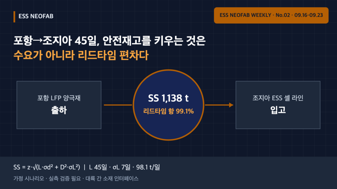
45 Days from Pohang to Georgia — Safety Stock at an Intercontinental Cathode Interface Is Driven by Lead-Time Variability, Not Demand

Abstract

On 22 September 2026, SK On signed an LFP cathode supply agreement worth about KRW 1.0742 trillion with POSCO Future M; volumes for 2027–2029 will go into ESS LFP cell manufacturing at SK On’s plant in Georgia, USA. To serve the contract, POSCO Future M has converted part of its high-nickel cathode line in Pohang to LFP and will start mass production at the end of this year. This means the interface¹ between the materials plant and the cell plant now spans a continent and an ocean crossing. Under an assumed scenario, about 99% of the safety stock at this interface is created not by demand variability but by lead-time variability. The management variable that shrinks the buffer is therefore not forecast accuracy but the standard deviation of the transport lead time.

1. Conclusion First — Lead-Time Variability Sets the Buffer at an Intercontinental Interface

Under the assumed conditions, the cathode safety stock in front of the Georgia cell line is about 1,138 t (about 11.6 days of supply), and 99.1% of it comes from the lead-time variability term. Halving the lead-time standard deviation from 7 days to 3.5 days nearly halves the safety stock to 577 t, whereas halving demand variability leaves it virtually unchanged at 1,136 t.

Situation (S): As sourcing non-Chinese cathode has become a priority in the ESS LFP cell supply chain, a structure has emerged in which cathode made in Korea is shipped to a US cell plant. Complication (C): Inter-process buffers inside a plant are usually designed in units of a few hours to one day, but here a transport leg of several weeks sits between the two plants. Question (Q): What determines the buffer size at this new interface? Answer (A): Lead-time variability, more than demand variability. The object of control is therefore not the cell line’s production plan but the spread of arrival times on the transport leg.

The assumption this article challenges is that “buffers exist because demand fluctuates.” That is broadly true for in-plant buffers. At an intercontinental interface with a long, variable lead time, however, the structure of the calculation changes.

2. Announced Facts and Assumed Conditions

The disclosed facts are as follows. The contract value is KRW 1,074,219,374,798 (per regulatory filing, 36.6% of recent revenue), and the supply period is the three years 2027–2029. The volumes will be used to manufacture ESS LFP cells at SK On’s Georgia plant, and POSCO Future M has converted part of the high-nickel line at its Pohang plant to LFP, with mass production starting at the end of this year. The two companies also plan to discuss extending supply beyond 2029.

Cathode unit price, cathode consumption per kWh of cell, and the capacity of the Georgia ESS line have not been disclosed. All figures below are therefore assumptions that require verification against contracts and actual measurements.

Item	Value	Basis
Annual contract value	about KRW 358.07 billion	Disclosed value ÷ 3 years (even split assumed)
Cathode unit price	KRW 8 / 10 / 12 million per t	Assumed scenarios (base: KRW 10 million/t)
Annual volume	44,759 / 35,807 / 29,839 t	Value ÷ unit price
Cathode consumption per cell	2.2 kg/kWh	Assumption
Equivalent cell capacity	20.35 / 16.28 / 13.56 GWh/yr	Volume ÷ consumption
Daily consumption (base)	98.1 t/day	35,807 t ÷ 365 days
Door-to-door lead time L	45 days	Assumption (Pohang shipment → Georgia receipt)
Lead-time standard deviation σL	7 days	Assumption (early operating period)
Daily demand standard deviation σd	9.81 t/day (coefficient of variation 10%)	Assumption

If the price assumption moves by ±20%, equivalent cell capacity ranges from 13.56 to 20.35 GWh/yr. The range is wide, but the conclusion below (the composition of the safety stock) holds regardless of the absolute volume.

3. Mechanism — Splitting the Safety-Stock Formula into Two Terms

When both demand and lead time vary, safety stock is written as follows.

SS = z × √( L·σ_d² + D²·σ_L² )

Here D is daily consumption and z is the service-level factor (1.65 for 95%). The first term under the root is the demand-variability term; the second is the lead-time-variability term. With base conditions, the demand term is 45 × 9.81² ≈ 4,330 and the lead-time term is 98.1² × 7² ≈ 471,576. The second term is about 109 times the first.

Scenario	Safety stock (t)	Days of supply	Share of lead-time term
Base (σL 7 days, CV 10%)	1,138	11.6 days	99.1%
Lead-time variability halved (σL 3.5 days)	577	5.9 days	96.5%
Demand variability halved (σd ÷ √2)	1,136	11.6 days	99.5%

Halving demand variability reduces safety stock by only 2 t. Halving lead-time variability reduces it by 561 t. The same “halving” delivers roughly a 280-fold difference in effect between the two management variables, and that is the core of this interface.

In-transit (pipeline) inventory comes on top. D × L = 98.1 × 45 ≈ 4,415 t, meaning about 12.3% of annual volume is always at sea or in port. Unlike safety stock, this inventory does not shrink when variability is reduced; it shrinks only when the mean lead time is shortened.

4. Line-Level Implications — Buffer Location and Cell-Line Takt Time

Converted to cells, 1,138 t of safety stock is about 0.52 GWh, or about 11.6 days of cell-line output. That is an order of magnitude larger than the in-plant practice of designing inter-process buffers at a few hours to one day. Where this inventory sits changes how the cell line operates.

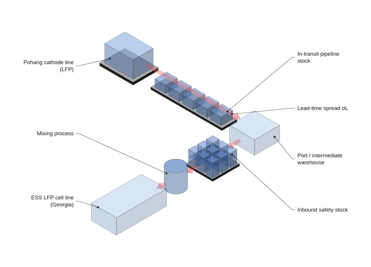
• Concentrated at the cell plant’s receiving warehouse: the risk of raw-material shortage in front of mixing is lowest. In exchange, warehouse space and moisture-control burden move to the cell plant.
• Distributed to port or intermediate warehouses: the space burden on the cell plant falls, but an additional inland transport leg is created and the lead-time variability term grows again.

The cell line’s takt time² is defined as available operating time ÷ customer demand and is set independently of material arrival variability. But when safety stock is insufficient, shortages reduce available operating time itself and destabilise the effective takt time. In other words, intercontinental lead-time variability is translated into availability loss on the cell line.

It also matters that the Pohang line has just been converted from high-nickel to LFP. Early after a conversion, the spread of shipment quality and schedule can widen, which pushes σ_L up. A reasonable approach is to set σ_L conservatively and hold a larger safety stock in the first year, then reduce it step by step using measured arrival data. This is an operating hypothesis that requires further verification.

Prior art includes a method for setting safety stock by quantifying the effect of mixed-model lines, demand-visibility horizons and lead times on each item’s optimal service level (US8315923B2). The formula in this article is simpler; its purpose is to show which term dominates when applied to an intercontinental materials interface.

5. Limitations and Scope

This calculation assumes that demand and lead time are independent and normally distributed. Actual ocean-freight delays often show a long right tail (port congestion, weather), so the normal assumption may underestimate safety stock. Also, because unit price, consumption and lead time are all assumptions, the absolute figures (t, days) must be replaced with contract and logistics measurements.

The direction of the conclusion, however — when lead time is long and σ_L is several days, the lead-time variability term dominates — does not depend on the price assumption. With a constant coefficient of variation, both terms scale with D², so their ratio reduces to σ_L² ÷ (L × CV²) and is independent of volume D. Under base conditions this value is 49 ÷ (45 × 0.01) ≈ 109.

FAQ

Q. Isn’t 10% demand variability too low?

Even if demand variability is tripled to 30%, the demand term is about 38,970, only about 8% of the lead-time term (471,576). Safety stock then becomes about 1,179 t, 3.6% above the base case. A larger demand-variability assumption does not change the conclusion.

Q. With a long-term contract, volumes are fixed — so isn’t safety stock unnecessary?

Fixed contract volumes do not fix arrival times. Almost all of the safety stock in this article comes from the spread of arrival times (σ_L), so fixing volumes contributes almost nothing to reducing the buffer. Reducing it requires managing lead-time spread through shipping frequency, carrier diversification and sharing of arrival data.

Field Application Notes

Check	How to execute	Remarks
☐ Obtain measured door-to-door lead-time history	Record shipment and receipt dates per recent shipment and compute mean L and σL	20+ samples recommended; separate seasonal variation
☐ Calculate the two safety-stock terms separately	Compute L·σd² and D²·σL² separately and record their shares	If the lead-time term is 90%+, the object of control is logistics
☐ Manage pipeline inventory separately	Separate D × L as in-transit inventory in financial and production planning	Does not shrink through variability control
☐ Agree on how shortage stops are recorded as availability loss	Record raw-material shortage stops under a code separate from equipment breakdowns	Prevents misattribution of OEE losses
☐ Set σL conservatively after a supplier line conversion	For the first year after the supplier’s conversion, set σL above measured values and recalculate quarterly	Operating hypothesis requiring further verification

---

Footnotes
¹ Interface: The boundary where different processes, equipment or plants exchange material and information. Here it refers to the boundary between cathode-plant shipment and cell-plant receipt.
² Takt Time: Available operating time ÷ customer demand. Not to be confused with Cycle Time or FPY.

Sources: Financial News (Korea), “SK On secures KRW 1.1 trillion of LFP cathode from POSCO Future M” (2026-09-22). POSCO Future M regulatory filing contract value (KRW 1,074,219,374,798; 36.6% of recent revenue). Prior-art reference patent (no new patents were found in the most recent 7 days, so the search was extended to 30 days; no newly published items were confirmed in that window either, so the patent is cited as general prior art only): US8315923B2 (Method of determining safety stock levels, published 2012-11-20).

Measurement and calculation conditions: Even annual split of contract value, unit price KRW 8/10/12 million per t, consumption 2.2 kg/kWh, lead time 45 days, σ_L 7 days, demand CV 10% and service level 95% (z = 1.65) are all assumptions. The comparison baseline is the ‘Base’ row of Table 2. Temperature, humidity, sample size and similar measurement conditions are not applicable (calculation scenario). Not to be cited for finalising inventory policy without measured verification.

---

Other Articles in This Issue

ESS NEOFAB WEEKLY No.02 · Research window 2026-09-16 to 2026-09-23

• A 25-Year Contract Increases Migrations, Not Storage — Traceability Design for Jeju Long-Term ESS Contracts (2026-09-24)
• A 2.5 GWh Line Fed Only 1 GWh of Cells — OEE of 36.9% and 83.8% Describe the Same Line (2026-09-25)