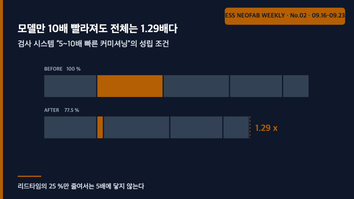
Even a tenfold faster model moves the whole by 1.29x — what “5 to 10 times faster commissioning” actually requires

Abstract

On 18 September 2026 Siemens and P&G announced that the AI-based quality inspection platform Visual Inspection Cockpit (VIC) is being rolled out across P&G’s manufacturing sites worldwide, stating that new deployments can be commissioned¹ five to ten times faster than traditional bespoke vision systems. Re-examining that figure through the structure of Amdahl’s law² inverts the received reading. Even if the AI model stage alone were ten times faster, total line lead time would fall only by a factor of 1.29 (22.5 %). For the announced 5× to hold, the accelerated portion must be at least 88.9 % of the lead time; and achieving 10× with a partial speed-up of 5 is arithmetically impossible. What the announcement actually describes, then, is not model reuse but standardisation of everything around the model — lighting, mechanics, integration and handover. The bottleneck in deploying an inspection system was never the AI.

1. The conclusion first — “5 to 10 times” does not mean the model got faster

Situation. VIC, the edge-based inspection platform jointly developed by Siemens and P&G, has finished pilot deployment and is expanding across P&G’s global manufacturing organisation³. Two results were published: a 10–20 % reduction in scrap rate depending on the product line, and a 5–10× reduction in commissioning time for new deployments.

Complication. The two figures are of entirely different natures. Scrap rate is in-service performance; the commissioning multiple is deployment lead time. Yet coverage and industry reaction bundle them into “the AI got faster, so deployment got faster.” That reading has never been verified.

Question. If AI model development accounts for less than half of the lead time of an inspection deployment, can the whole ever shrink by 5–10× no matter how fast the model becomes?

Answer. It cannot. The contribution of a partial optimisation to the whole has a ceiling — Amdahl’s law — and that ceiling does not yield to any choice of assumed values. If the published figures are accurate, what was shortened is not the model but very nearly the entire lead time. And that “very nearly all of it” contains items that have nothing to do with AI.

2. What was published, and what was not

Item	Published	Not published
Platform composition	P&G’s proprietary deep learning models + consumer-goods manufacturing domain knowledge / Siemens edge computing hardware, software scaling frameworks, industrial AI portfolio	Model architecture, edge hardware specification
Inspection performance	Real-time inspection during production, full inspection coverage at full line speed	Absolute line speed (m/min), resolution, minimum defect size (mm)
Quality result	Scrap rate reduced 10–20 % depending on product line	Whether the baseline is the existing in-house vision system or no inspection
Deployment result	New deployments commissioned 5–10× faster (versus traditional bespoke vision systems)	The scope of what was shortened — whole line, or only the model deployment stage
Rollout scope	P&G manufacturing sites worldwide	Number of sites, rollout schedule

This article reads the commissioning multiple as applying to whole-line lead time. The original text does not state the scope, so this is an interpretation; if the actual scope is only the model deployment stage, the back-calculation in Section 4 does not hold. That condition is stated up front.

3. Decomposing the lead time — the model is one quarter

Set up an assumed scenario. The lead time to deploy a bespoke vision system on one new line is decomposed as below. These are arbitrary values based on field observation and must be replaced with your own records and recalculated.

Stage	Content	Share of lead time (assumed)	Shortened by model reuse?
①	Requirements, defect definition, sample collection	20 %	Partly — only where the defect definition is unchanged
②	Model training and tuning	25 %	Yes
③	Lighting, optics, mechanical installation	25 %	No
④	On-site integration, commissioning, validation	20 %	No
⑤	Operational handover and documentation	10 %	No

Now apply Amdahl’s law. Where a portion of share f is accelerated by a factor s, the overall speed-up S is

S = 1 ÷ [ (1 − f) + f ÷ s ]

Accelerated portion	f	Partial factor s = 5	s = 10	s = ∞ (instantaneous)
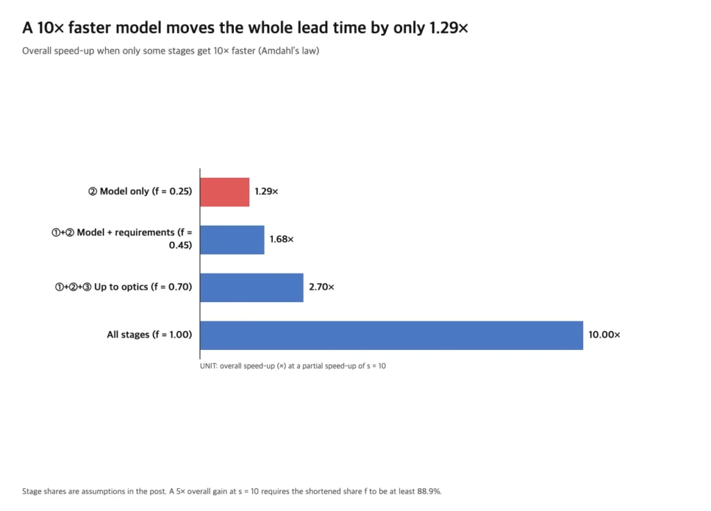
② model only	0.25	1.25× (20.0 % ↓)	1.29× (22.5 % ↓)	1.33× (25.0 % ↓)
①+② model and requirements	0.45	1.56× (35.9 % ↓)	1.68× (40.5 % ↓)	1.82× (45.0 % ↓)
①+②+③ including optics	0.70	2.27× (56.0 % ↓)	2.70× (63.0 % ↓)	3.33× (70.0 % ↓)
everything	1.00	5.00× (80.0 % ↓)	10.00× (90.0 % ↓)	—

The first row of Table 3 is this article’s starting point. Accelerating model training tenfold shortens total lead time by only 22.5 %. That is an order of magnitude away from the announced 5–10×. Making the model infinitely fast still yields no more than 25 %, because the remaining 75 % is untouched.

4. Back-calculation — 5× requires a scope of 88.9 % or more

Reverse the direction. To achieve a target overall factor S, what must f be? Solving the expression above for f gives

f = (1 − 1÷S) ÷ (1 − 1÷s)

Target overall factor S	Partial factor s = 5	s = 10	s = 20	s = ∞
5×	f = 100.0 %	f = 88.9 %	f = 84.2 %	f = 80.0 %
10×	f = 112.5 % — arithmetically impossible	f = 100.0 %	f = 94.7 %	f = 90.0 %

Three things follow.

First, even 5× requires f ≥ 80 %. That holds however large the partial factor s becomes. “Five times faster commissioning” therefore means at least four fifths of the lead time was addressed, and ② alone (25 % in Table 2) can never get there.

Second, achieving 10× with a partial factor of 5 is arithmetically impossible, since it yields f = 112.5 % and no share exceeds 100 %. If the published upper figure of 10× is accurate, the scope must be everything and the partial factor must simultaneously be 10 or more.

Third, what then shortened ③④⑤? The answer is already in the announcement — what Siemens supplied was not a model but edge computing hardware and software scaling frameworks³. When the hardware is standardised, ③ (lighting, optics, mechanics) is no longer designed from scratch each time; with a scaling framework, ④ (on-site integration and commissioning) becomes a deployment procedure; and on an identical platform, ⑤ (handover and documentation) reduces to a copy. In this structure AI is not the cause of the shortening but merely one of the things that standardisation made possible.

5. Separating the layers — in-service performance and deployment lead time are different problems

The earlier piece on this site covering the dual constraint of bandwidth versus takt time in inline 3D inspection dealt with what hits the limit first while an inspection system is running. This article deals with what consumes time while that system is being brought in. The two calculations are independent. A design with ample bandwidth and latency budget can still take eighteen months to deploy, and conversely a system deployed in a day may fail to keep up with full line speed. When an inspection investment is reviewed, both tables should be demanded separately.

The scrap-rate side needs its own layer distinction too. How that reduction shows up in OEE⁴ is handled separately in the FAQ, but to state the conclusion first: the OEE improvement is under 0.4 %p, and the payback comes not from OEE but from material cost and waste disposal cost. The general structure of marginal contribution by OEE factor was already decomposed in the piece on marginal capacity gain across the three OEE levers under an approval freeze, and is not repeated here.

FAQ

Q1. The shares in Table 2 are arbitrary — can the calculation built on them be trusted?
If Table 2 changes, the figures in Table 3 change. Table 4, however, does not. Table 4 is a relation between target factor and required f, and does not depend on the decomposition. This article’s core claims — “5× requires f ≥ 80 %”, “10× is impossible at s = 5” — hold irrespective of the assumed values. All Table 2 does is present the circumstantial case that the real f is likely to fall well short of 80 %; if that circumstance is wrong, the rebuttal has to take the form of your own decomposition from records. That is item 1 of the field application notes.

Q2. Surely a 20 % scrap reduction lifts OEE appreciably?
It does not. Assuming a baseline scrap rate of 2.0 %, a 20 % reduction gives 1.6 % and a quality factor Q of 98.0 % → 98.4 %. Against a baseline of 88 % availability and 92 % performance, OEE moves 79.34 % → 79.67 %, that is +0.32 %p. A 10 % reduction yields only +0.16 %p. Material saved, by contrast, is directly proportional to scrap volume, so the material-cost effect receives the full 20 %. Submit this investment on the grounds of OEE improvement and the number looks trivial; submit it on material and waste disposal cost and it is honest. (Measurement conditions: baseline scrap 2.0 %, A 88 % and P 92 % are all assumed values, and the baseline was set identical to the earlier article for comparability.)

Q3. Does this mean AI inspection deployment is not worth much?
The opposite. What this analysis points to is changing the question asked at investment review. “What is the model accuracy?” bears on ② alone, whereas what determines 75 % of the lead time is whether the lighting and mechanics are standard parts, whether the integration procedure is documented, and whether acceptance criteria are already agreed. If a platform solution looks expensive, the calculation must include that what its price contains is not the model but the standardisation of ③④⑤.

Field application notes

Only items that can be started on Monday morning are listed.

#	Action	Output	Effort
1	Decompose the actual lead time of your two or three most recent vision deployments in the format of Table 2 — start date, model freeze date, mechanical installation completion, commissioning completion, acceptance date.	Your own measured f	1 day
2	Substitute that f into Table 4 and determine whether a 5× reduction is even sayable at your plant. If f < 0.80, no solution can deliver 5×.	1-line determination	0.5 day
3	Confirm in writing with suppliers the scope of the commissioning multiple — whole line, or model deployment stage only. That single sentence changes the basis on which proposals compare.	1 enquiry	0.5 day
4	For the two stages with the largest share (usually ③ optics and mechanics, ④ integration and commissioning), check whether in-house standard parts and standard procedures exist. Where they do not is the real improvement point.	Standardisation gap list	1 day
5	Replace the benefit line of the inspection investment case from OEE to material and waste disposal cost and recompute the amount.	Revised investment basis	0.5 day

Sources and measurement conditions

¹ Commissioning — the sequence of testing, adjustment and verification from installation of equipment through confirmation that it meets specified performance and handover to the operating organisation. This article uses the announcement’s own word “commissioned”.
² Amdahl’s law — the relation stating that improving only part of a whole places an upper bound on the improvement of the whole. It originated in parallel computing but applies in the same form to any problem expressible as a sum of serial stages.
³ Siemens press release, “Siemens and Procter & Gamble roll out AI-based quality inspection worldwide”, 18 September 2026. Carried identically by AIwire, Industry EMEA and WebWire among others. Source for all items in Table 1 and for the “edge computing hardware and software scaling frameworks” statement in Section 4.
⁴ OEE (Overall Equipment Effectiveness) — availability × performance × quality. This site fixes that definition and does not conflate it with cycle time or FPY.

Basis of calculation. The stage shares in Table 2, the baseline scrap rate of 2.0 %, and availability 88 % / performance 92 % are all assumptions stated in the body text. The relation in Table 4 does not depend on assumed values. The measurement period, sample size and product lines behind the published figures are not disclosed in the original and are therefore not reflected.

Patent note. No relevant patent was published within this issue’s research window (16–23 September 2026); the search was extended to 30 days and again returned none. The following are offered as general prior art only, with no claim of direct correspondence to this subject.

• US11120306B2 — Edge-based adaptive machine learning for object recognition (published 2021-09-14)
• US11544566B2 — Deep learning model insights using provenance data (published 2023-01-03)

Also in this issue

• Why three qualified products landed on the same duration — in DSX Ready BESS, sizing is set by the output axis
• 16 GWh committed and 190 GWh reserved — what absorbs the 2.97x step is the contract, not the line