If Availability, Performance and Quality Are All 80 %, OEE Is 51.2 % — How to Calculate OEE
Abstract
OEE (overall equipment effectiveness) is calculated as availability × performance × quality, and the Japan Institute of Plant Maintenance (JIPM) gives the example that when all three factors are 80 %, OEE is 51.2 %¹. When the three factors are multiplied as JIPM defines them, OEE is organized as “standard (planned) cycle time × number of good units ÷ loading time,” that is, the share of loading time spent making good units at the standard speed². In an assumed shift (loading time 27,600 s, standard cycle time 32 s, 690 good units), availability is 90.0 %, performance 90.4 % and quality 98.3 %, giving an OEE of 80.0 %. If loading time equals the available working time used for takt time, the minimum OEE needed to meet demand is calculated directly as “standard cycle time ÷ takt time.”
1. Conclusion First — OEE Is the Product of Three Ratios, and Expanding the Product Yields a One-Line Formula
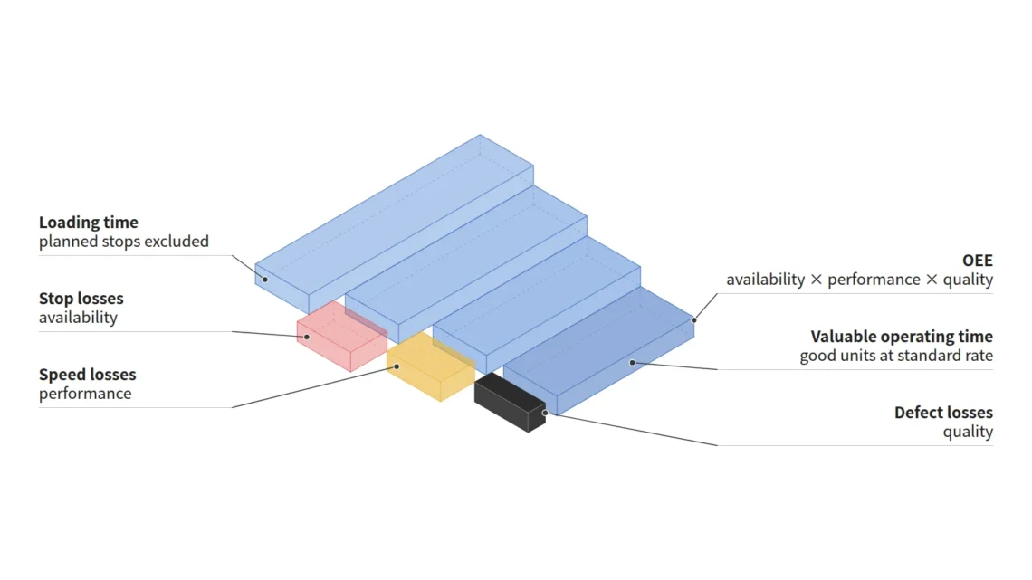
The conclusion comes first. OEE is the value obtained by expressing stop loss (availability), speed loss (performance) and defect loss (quality) each as a ratio and then multiplying them. When the product is expanded, the intermediate terms cancel and only “standard cycle time × number of good units ÷ loading time” remains². OEE can therefore be cross-checked with three numbers, without aggregating the three factors separately.
Situation (S): JIPM introduces OEE as a representative indicator of equipment maintenance, centered mainly on automated lines³. Complication (C): because of the multiplicative structure, OEE falls substantially even when each factor looks high, and the names and denominators of the factors differ from one standard to another. Question (Q): what are the three factors calculated from, and on what basis should different OEE values be compared? The answer (A) is given in the mapping table below and in Sections 2–5.
| Term on this site | JIPM term | ISO 22400-2 (OPC restatement) | Formula (JIPM basis) |
|---|---|---|---|
| Availability | Time availability rate (時間稼働率) | Availability = APT ÷ PBT | (Loading time − stop time) ÷ loading time |
| Performance | Performance rate (性能稼働率) | Effectiveness = PRI × PQ ÷ APT | (Standard cycle time × processed quantity) ÷ operating time |
| Quality | Quality products rate (良品率) | Quality rate = GQ ÷ PQ | Number of good units ÷ input quantity |
| OEE | Overall equipment effectiveness (設備総合効率) | Product of the three values | Standard cycle time × number of good units ÷ loading time |
※ The ISO formulas are restated from an OPC Foundation document that cites ISO 22400-2, and the OEE clause of the ISO original (Clause 6) lies in the paywalled body text and could not be verified directly⁴·⁵. Abbreviations: APT, actual production time; PBT, planned busy time (= planned operation time POT − planned downtime); PRI, planned runtime per item; PQ, produced quantity; GQ, good quantity. The JIPM TPM Excellence Award examination guidelines use 計画サイクルタイム and the pe-digital series uses 基準サイクルタイム; this article treats the two as the same value and unifies them as “standard cycle time” (an interpretation; the body text defining 基準サイクルタイム is members-only and was not verified).
2. Calculating the Three Factors — From Loading Time to Good Units
The starting point is loading time (負荷時間). JIPM defines loading time as working time minus the time for which stopping the equipment has been scheduled in advance, such as planned construction and maintenance work, pre-start inspections, morning meetings and breaks⁶. Operating time (稼働時間) is loading time minus the time the equipment was stopped by breakdowns or setup and adjustment, that is, the time the equipment actually ran⁶.
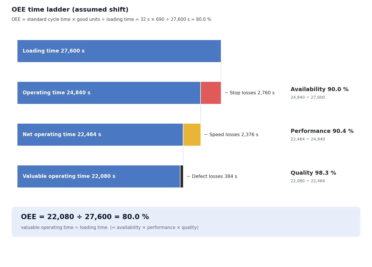
The three factors are calculated by stepping down this time ladder one rung at a time. Availability (time availability rate) is (loading time − stop time) ÷ loading time⁶. Performance (performance rate) is (standard cycle time × processed quantity) ÷ operating time, and JIPM describes it as an indicator that reveals the size of speed-reduction loss and minor-stoppage loss²·⁶. Quality (quality products rate) is the number of good units ÷ input quantity, where the number of good units is the input quantity minus defects at start-up and during trial processing, in-process defects and the quantity corrected or reworked⁶.
| Step | Value (assumed) | Calculation | Result |
|---|---|---|---|
| Loading time | 27,600 s | Shift 28,800 s − planned breaks 1,200 s | — |
| Stop time (breakdowns, setup and adjustment) | 2,760 s | — | — |
| Operating time | 24,840 s | 27,600 − 2,760 | Availability 90.0 % |
| Standard cycle time × processed quantity | 32 s × 702 units = 22,464 s | 22,464 ÷ 24,840 | Performance 90.4 % |
| Number of good units ÷ input quantity | 690 units ÷ 702 units | 690 ÷ 702 | Quality 98.3 % |
| OEE | — | 0.900 × 0.904 × 0.983 | 80.0 % |
| Cross-check | — | 32 × 690 ÷ 27,600 | 80.0 % |
※ Calculation conditions: 1 shift; all figures are assumed values for illustration, and the processed quantity and the input quantity are assumed to be equal at 702 units. Expressed as time, the losses are 2,760 s of stops, 2,376 s of speed loss and 384 s of defects (12 units × 32 s), and the remaining 22,080 s is the time spent making good units at the standard speed. Implication: because the product of the three factors and “standard cycle time × number of good units ÷ loading time” must be equal, a mismatch between the two values in an aggregation system signals an error somewhere in the aggregation rules.
3. The Illusion Created by Multiplication — Three Factors at 80 % Give 51.2 %
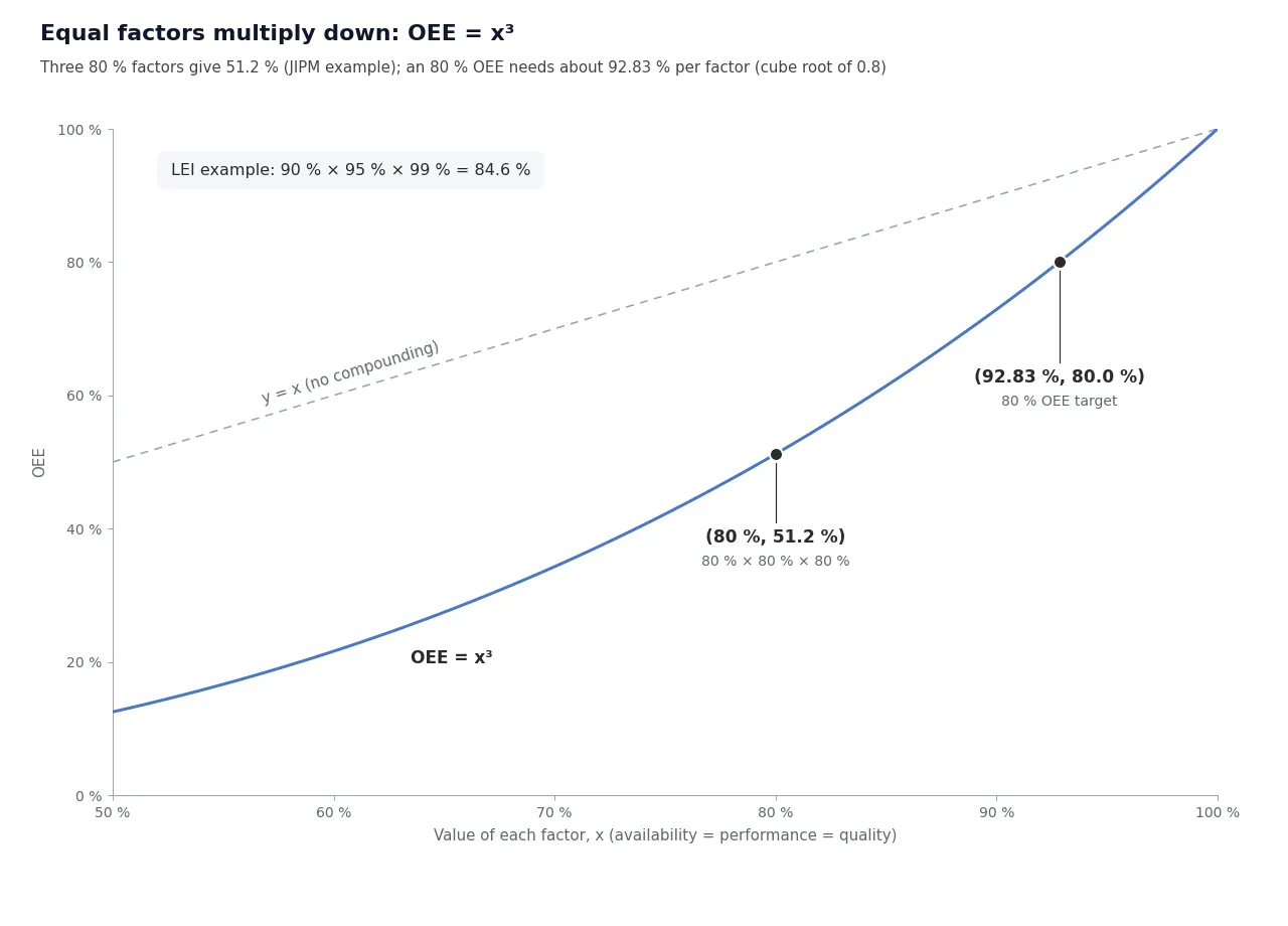
The multiplicative structure lowers the value faster than intuition suggests. JIPM illustrates that when the time availability rate, performance rate and quality products rate are all 80 %, OEE is 0.8 × 0.8 × 0.8 = 0.512, or 51.2 %¹. The example in the LEI (Lean Enterprise Institute) glossary likewise calculates OEE as 84.6 % at availability of 90 %, performance of 95 % and quality of 99 %⁷.
| Three factors (same value) | OEE |
|---|---|
| 80 % | 51.2 % |
| 85 % | 61.4 % |
| 90 % | 72.9 % |
| 92.83 % (cube root of 0.8) | 80.0 % |
| 95 % | 85.7 % |
※ Calculation conditions: a simple calculation for the case in which all three factors have the same value (OEE = x³). Implication: distributing an OEE of 80 % evenly across the three factors requires each factor to be about 92.83 % (the cube root of 0.8).
Conversely, the loss structure can differ even when the OEE is the same. As an assumed example, a line with all three factors at 90 % and a line with availability of 81 %, performance of 100 % and quality of 90 % both have an OEE of 72.9 %. In the former the losses are spread evenly, whereas in the latter the stop loss is large, so a single OEE figure cannot determine what to improve.
4. Names and Denominators Differ by Standard — JIPM, ISO 22400-2, SEMI E79
OEE is not unified under a single formula. JIPM uses loading time as the denominator⁶, while ISO 22400-2 uses planned busy time (PBT), that is, planned operation time (POT) minus planned downtime, as the denominator of availability⁴·⁵. The 2019 revision draft (Draft Document 6579, an Informational Ballot for comments) of the semiconductor equipment standard SEMI E79 defines OEE as “theoretical production time for effective units ÷ total time” and states that it can also be calculated as the product of four efficiencies: availability, operational, rate and quality⁸.
| Source | Name | Denominator | Number of factors | Scope verified in this article |
|---|---|---|---|---|
| JIPM | 設備総合効率 | Loading time | 3 | Institute’s public articles; TPM Excellence Award examination guidelines (受審要領) |
| ISO 22400-2:2014 | overall equipment effectiveness | PBT | 3 (Availability, Effectiveness, Quality) | Preview definitions + OPC restatement |
| SEMI E79 | overall equipment efficiency | total time | 4 | 2019 revision draft (Informational Ballot; body text of the current E79-0422 not verified) |
| LEI glossary | Overall Equipment Effectiveness | scheduled time | 3 | Glossary entry |
※ The names also diverge. ISO defines OEE as the abbreviation of overall equipment effectiveness⁴, SEMI uses overall equipment efficiency⁸, and JIPM materials contain both expressions¹·³. Implication: OEE values with different denominators cannot be compared directly, so the denominator and the period must be stated next to any OEE value.
The Korean national standards framework is also worth confirming. ISO 22400-2 was adopted as an identical (IDT) Korean standard, KS X ISO 22400-2, established on 2024-12-13⁹. Meanwhile, ISO 22400-2:2014 is at the “to be revised” stage at ISO and a draft of the 2nd edition (ISO/DIS 22400-2) is under development¹⁰, so the definition clauses must be checked again once the revised edition is published.
Problems surrounding the denominator have already been discussed on this site. A 2.5 GWh Line Fed Only 1 GWh of Cells — OEE of 36.9% and 83.8% Describe the Same Line dealt with where material shortage (cell starvation) time should be classified, and StarPlus Energy’s Indiana Plant — The Blended-OEE Illusion Created by Sequential NCA/LFP Commissioning dealt with the illusion that arises when several lines are aggregated. This article is the foundational installment that sets out the premises of both discussions: how the three factors are calculated and how the definitions differ between standards.
5. Linking to Takt Time — Minimum Required OEE = Standard Cycle Time ÷ Takt Time
Writing OEE as “standard cycle time × number of good units ÷ loading time” ties it directly to the demand condition. Because the number of good units in a shift must be at least equal to demand, OEE ≥ standard cycle time × demand ÷ loading time. If loading time is assumed to equal the available working time in the takt time calculation, loading time ÷ demand is the takt time itself, so minimum required OEE = standard cycle time ÷ takt time. This one line is the new formula that this article adds.
| Standard cycle time (assumed) | Takt time | Minimum required OEE |
|---|---|---|
| 28 s | 40 s | 70.0 % |
| 32 s | 40 s | 80.0 % |
| 36 s | 40 s | 90.0 % |
※ Calculation conditions: the takt time of 40 s is the LEI textbook example used in Part 1 of this series (available working time 27,600 s, demand 690 units), and the standard cycle times are assumed values. The assumed shift in Section 2 has an OEE of exactly 80.0 % and therefore just meets the demand of 690 units. Implication: an OEE target should be set starting from its lower bound, the ratio of standard cycle time to takt time, and if the two time bases differ (for example, when changeover is subtracted from loading time), this formula needs correction.
In summary, there are three points. Because OEE is the product of three factors, it can fall substantially even when each factor looks high. Expanding the product gives standard cycle time × number of good units ÷ loading time, which makes cross-checking and target setting easier. The denominator and the name, however, differ by standard, so the definition must be stated alongside any comparison.
The limitations are equally clear. The OEE clause of ISO 22400-2 and the body text of the current edition of SEMI E79 are paywalled and could not be verified directly; the ISO formulas rest on the OPC Foundation restatement and the SEMI formulas on the 2019 revision draft (Informational Ballot). The premise that loading time = available working time must be confirmed against each line’s definition document, and because all example values are assumed, further verification against measured data is needed.
FAQ
Q1. Where does the benchmark that an OEE of 85 % is “world class” come from?
This benchmark could not be found in the primary sources consulted (the publicly available portion of ISO 22400-2, JIPM, SEMI and the LEI glossary). LEI’s 84.6 % is a value presented as a calculation example⁷, and JIPM, while stating that a higher OEE is better, writes that targets and benchmarks differ depending on the product, the production process, the newness of the equipment and other factors¹. A target set from its lower bound under the demand condition, as in Section 5, rests on a clearer basis.
Q2. Isn’t it enough to manage availability (time availability rate) alone?
By JIPM’s definition, the time availability rate is an indicator that evaluates the size of stop losses such as breakdowns or setup and adjustment². Speed reduction and minor stoppages surface in the performance rate, and defects and rework surface in the quality products rate²·⁶. As with the two lines in Section 3, looking at only one factor hides the other losses.
Q3. If two lines have the same OEE, can their results be regarded as equal?
Only when the denominator and the classification rules are the same. As Section 4 shows, the denominator differs by standard, and even within one standard the value changes depending on where material shortage and changeover time are placed (see the calculation in Part 4 of this series). A comparison table should state the denominator, the period and the classification rules together with the OEE.
Field Application Notes
| Check | How to execute | Decision criterion | Remarks |
|---|---|---|---|
| ☐ Write a 1-page OEE definition sheet | Document the list of planned downtime to subtract from loading time, the source of the standard cycle time and the good-unit judgment (whether reworked units are included) | Is the definition identical across lines? | Differences between standards (Section 4) |
| ☐ Cross-check with three numbers | Compare standard cycle time × number of good units ÷ loading time with the product of the three factors | The two values match | If they differ, inspect the aggregation rules |
| ☐ Break down loss time | Express stop, speed and defect losses in s (Section 2 method) | Select 1 largest-loss item | Improvement priority |
| ☐ Calculate the minimum required OEE | Standard cycle time ÷ takt time | Actual OEE ≥ lower bound | Premise: loading time = available working time |
| ☐ Revise the reporting format | State the denominator, period and classification rules next to the OEE | 0 reports without them | Measurement-condition notes |
Sources and Notes
¹ 公益社団法人日本プラントメンテナンス協会(JIPM), 「指標でモノづくりを評価しよう! #1 設備総合効率(OEE)」, pe-digital.jp, 2025-04-01, pe-digital.jp. The definition sentence, the formula, the 80 % example (0.8×0.8×0.8=0.512) and the sentences on targets and benchmarks are cited.
² JIPM, 「2021年度 TPM®優秀賞 ②受審要領(国内事業場 最終版)」 “1. 活動の効果指標” pp.20–21, jipm.or.jp PDF. The 時間稼動率 formula and explanation, 設備総合効率 = 計画サイクルタイム × 良品数量 ÷ 負荷時間 × 100, and the 性能稼動率 explanation are cited.
³ JIPM, 「TPMとは」, info-jipm.jp. Describes OEE as a representative indicator of equipment maintenance centered on automated lines (English notation: Overall Equipment Efficiency).
⁴ ISO 22400-2:2014, Automation systems and integration — Key performance indicators (KPIs) for manufacturing operations management — Part 2, Edition 1 (2014-01-15), preview. The Clause 3 abbreviations, 5.1.2.2 POT, 5.1.2.4 PBT, 5.1.3.6 APT and the table of contents (Clause 6 KPI descriptions, Annex B) are cited. Clause 6, which contains the OEE formula, was not verified.
⁵ OPC Foundation, OPC UA for Machine Tools Part 1, Annex C.2 “KPI Calculation” and C.2.4 “Calculation of the OEE,” reference.opcfoundation.org. A restatement that cites the ISO 22400-2 definitions (not the ISO original).
⁶ JIPM, pe-digital.jp series 「指標でモノづくりを評価しよう!」, part 2 時間稼働率 (2025-05-12), part 3 性能稼働率 (2025-06-18) and part 4 良品率 (2025-07-10), publicly available portions. The definitions of loading time and operating time and the formulas for the performance rate and quality products rate are cited.
⁷ LEI, Lean Lexicon entry “Overall Equipment Effectiveness,” lean.org. The formula, the 84.6 % example, the explanation of availability and the 6 big losses are cited.
⁸ SEMI, Draft Document 6579(Revision to SEMI E79-0814E) Informational Ballot, 2019-10-25, 8.1.1 and 8.1.2, Eq.18–20. The scope statement on the store page of the current edition, SEMI E79-0422, was referenced; its body text was not verified.
⁹ Korean Agency for Technology and Standards, e-나라표준인증 portal, KS X ISO 22400-2 standard information (established 2024-12-13, Notice 2024-0608, ISO 22400-2:2014 IDT), standard.go.kr.
¹⁰ ISO, ISO 22400-2:2014 standard information (90.92, to be revised) and ISO/DIS 22400-2 standard information (40.99, 2024-09-17), iso.org.
※ Assumed values: the shift of 28,800 s, planned breaks of 1,200 s, stops of 2,760 s, standard cycle times of 28, 32 and 36 s, and 702 processed units and 690 good units are illustrative assumptions and require verification against measured data.
Line Metrics Glossary — Other Articles in This Series
- Part 1. Don’t Subtract Breakdowns When Calculating Takt Time — Takt Time vs. Cycle Time vs. Lead Time
- Part 3. FAT and SAT Differ in More Than Location — How IEC 62381:2024 Defines the Tests
- Part 4. Is a Changeover Planned Downtime or an Availability Loss? — How the Definition Changes OEE


2 Comments
Pingback:
Pingback: