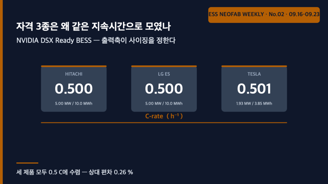
Why three qualified products landed on the same duration — in DSX Ready BESS, sizing is set by the output axis

Abstract. On 21 September 2026 NVIDIA launched DSX Ready, a qualification program for AI factory power and cooling products, and placed three BESS (Battery Energy Storage System) offerings on the initial qualified list. Converting the published ratings gives 0.500 C for Hitachi Energy, 0.500 C for LG Energy Solution and 0.501 C for the Tesla Megapack 2XL — a spread of 0.26 %. This convergence is not a coincidence. Of the three functions named in the qualification scope (load buffering, demand response, operation through grid disturbances), only demand response governs sizing; load buffering is satisfied automatically underneath that sizing, with an energy margin of 240×. The variable that site engineering actually has to argue about is therefore not energy capacity but PCS output and unit granularity — and the response-latency specification is absent from the public material, so it has to be confirmed separately.

1. The conclusion first — the qualified list tells you what governs sizing, not what you may buy

NVIDIA published DSX Ready on its own blog on 21 September 2026¹, and industry media reported the ratings of the three qualified BESS products a day later². The situation is clear: the selection of power and cooling equipment for AI factories is moving from individual procurement negotiation to prior qualification. The complication follows. The qualified list publishes product names and ratings only; it does not say which requirement those ratings were derived from.

The question is this. Three companies use different cells, PCS and packaging — so why did they converge on the same duration? The answer is simple. Of the three functions enumerated in the qualification scope, only demand response determines energy capacity; the other two demand output alone. That is why all three products landed on two hours (0.5 C). And that fact hands the site engineer one practical conclusion: almost any attempt to optimise energy capacity within this product class is wasted effort.

2. Published ratings — three products inside 0.26 % of the same duration

Supplier	Product	AC output	Energy	C-rate (derived)	Nominal duration (derived)
Hitachi Energy	WD4 PCS + battery storage	5.00 MW	10.00 MWh	0.5000 h⁻¹	2.000 h
LG Energy Solution	LGES Vertech JF2 2HR/4HR AC Link	5.00 MW	10.00 MWh	0.5000 h⁻¹	2.000 h
Tesla	Megapack 2XL	1.93 MW	3.85 MWh	0.5013 h⁻¹	1.995 h

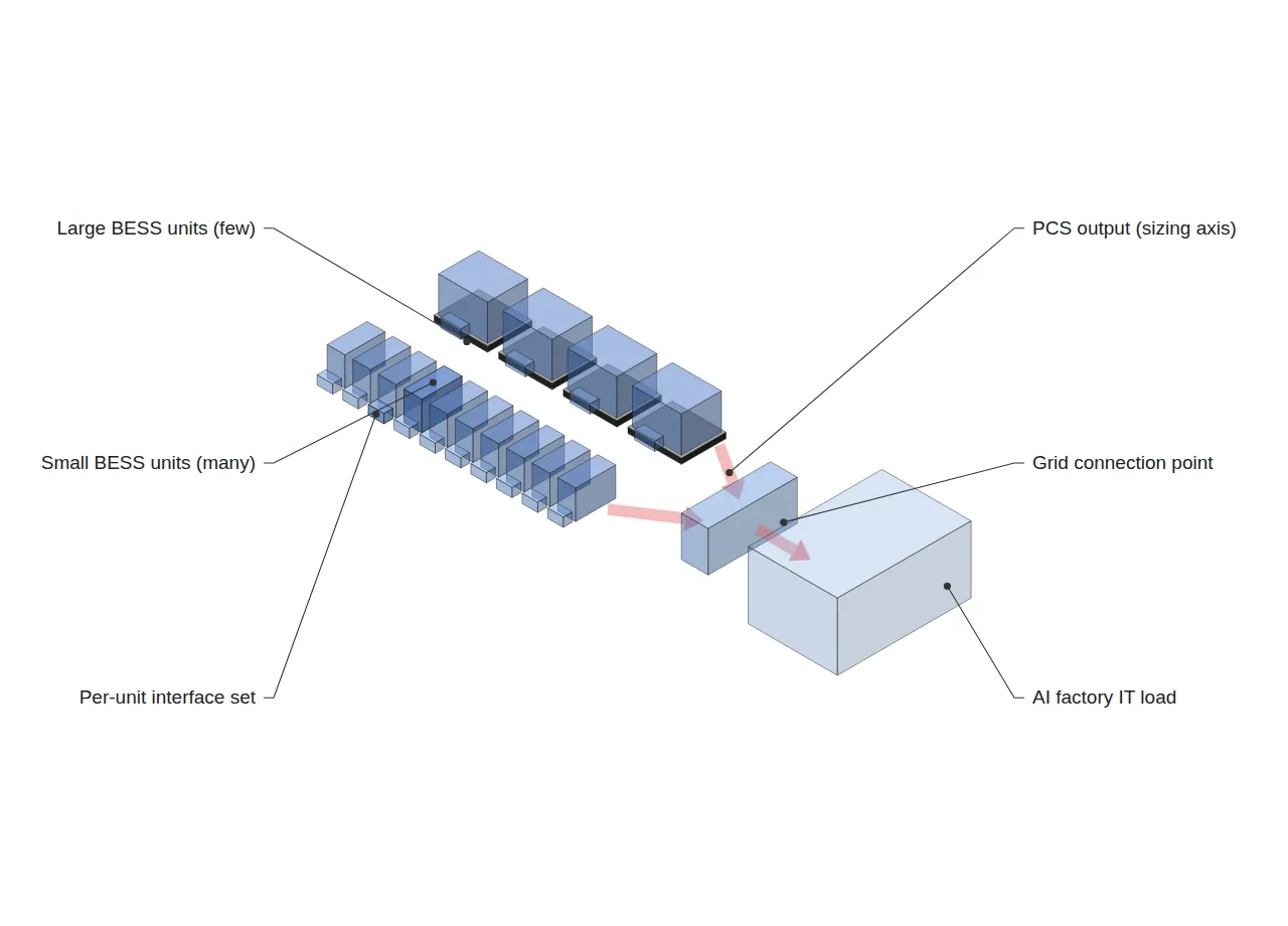
Two things stand out. First, the duration is effectively identical. Second, the unit granularity is not. 10.00 MWh and 3.85 MWh differ by a factor of 2.60. The three passed the same qualification, but the way they sit on a site is entirely different. It is worth recording that the LG Energy Solution product name carries “2HR/4HR” — a four-hour configuration exists, yet the published qualified rating is the two-hour one.

3. The sizing arithmetic — load buffering leaves 240× the energy unused

Set up an assumed scenario. The figures below are set arbitrarily to establish an arithmetic baseline; they must be replaced with actual site values and recalculated.

• AI factory IT load: 100 MW (assumed)
• Transient duration targeted by load buffering: 30 s (assumed)
• Duration targeted by demand response: 2 h (set equal to the nominal duration of the qualified product class)

Taking load buffering alone, the required energy is 100 MW × (30 s ÷ 3,600 s·h⁻¹) = 0.833 MWh. The required output remains 100 MW. But meeting 100 MW of output takes twenty 5 MW units, and those twenty units bring 200 MWh with them.

Function	Required output	Required energy	5 MW units needed	Energy that follows	Energy margin
Load buffering (30 s assumed)	100 MW	0.833 MWh	20	200 MWh	240.0×
Demand response (2 h assumed)	100 MW	200 MWh	20	200 MWh	1.00×
Operation through grid disturbances	100 MW	duration requirement not published	—	—	cannot be computed

What matters here is not the figure 240 itself but the structure that makes the margin free. Nobody buys energy separately for buffering. The moment the demand-response requirement is met, the buffering energy is exceeded 240-fold. Conversely, sizing to energy alone — a single 10 MWh unit — yields 5 MW of output, 5 % of the target. In a 0.5 C product class, sizing is set entirely by output, and energy is a dependent variable.

This conclusion also fixes where the four-hour configuration belongs. At equal energy a 4HR unit has half the output, so if the purpose is buffering or disturbance ride-through, the same output target takes twice as many units. The only case in which 4HR is justified is when the purpose is hour-scale energy shifting — demand response or tariff arbitrage.

4. Unit granularity — saving 1.5 %p of over-provisioning costs 160 % more interfaces

Return to the second observation from Table 1: 10.00 MWh versus 3.85 MWh, that is 5.00 MW versus 1.93 MW. When a target output P is divided by a unit output u, the expected surplus (over-provisioning) arising in the last unit can be taken as u/2, while the interface count is proportional to P/u. One interface is a single set of power connection, communications, fire protection and ventilation supply, and commissioning labour is directly proportional to it.

Target output P	5.00 MW unit — expected over-provisioning	1.93 MW unit — expected over-provisioning	Over-provisioning saved	Interface count (5.00 / 1.93)	Interface increase
20 MW	2.50 MW (12.5 %)	0.97 MW (4.8 %)	7.7 %p	4.0 / 10.4	+6.4 (+160 %)
100 MW	2.50 MW (2.5 %)	0.97 MW (1.0 %)	1.5 %p	20.0 / 51.8	+31.8 (+160 %)
200 MW	2.50 MW (1.3 %)	0.97 MW (0.5 %)	0.8 %p	40.0 / 103.6	+63.6 (+160 %)

There is one controlled variable here. The absolute saving in over-provisioning is fixed at 1.535 MW independently of P, because the surplus only ever arises in the last unit. The interface increase, by contrast, is 0.318 × P and therefore proportional to P. As scale grows, the advantage of the smaller unit stays constant while the burden grows — large sites favour large units; 20 MW-class sites and phased expansions favour small ones. The crossover scale is set by the ratio between commissioning labour cost per interface and capital cost per MW of over-provisioning; neither unit cost appears in the public material, so no figure is specified here (to be confirmed).

5. Qualification is an interface contract, not site engineering

NVIDIA states this itself. The original text explains that BESS partners run the required tests within a defined qualification boundary and submit supporting data for review, then makes the point explicitly: “Passing qualification does not replace site-level engineering or imply site-level stability.”¹ The same piece also notes that “optimizing one part of an AI factory can shift the bottleneck elsewhere.”¹ From a line- and system-integration standpoint the two sentences say the same thing. Qualification standardises the boundary conditions of a component, and the more the inside of that boundary is standardised, the more the remaining design freedom moves outside it — layout, clearances, supply and exhaust air, the point of grid connection, and unit granularity.

This article sits next to the earlier piece on station block scale-up and the commissioning interface budget, but at a different layer. That article decomposed how labour (time) behaves when block capacity grows; this one examines which axis constrains the rating (power and energy) of a qualified product class. The time axis and the rating axis are determined independently, and in practice both calculations are required.

Finally, the limits of this analysis should be stated plainly. The 30 s buffering duration is an assumption. If the actual transient runs to minutes, the energy margin collapses quickly: at 10 minutes 240× becomes 12×, and at 60 minutes it becomes 2×, at which point the output-dominated structure breaks down. The condition under which this article’s conclusion holds is that the target transient is sub-minute, and confirming that depends on measuring each site’s own load profile. Further verification is required.

FAQ

Q1. If there is 240× of margin, isn’t using the qualified product wasteful? Wouldn’t a separate 1 MWh high-output asset dedicated to buffering be cheaper?
Arithmetically, yes. Satisfying 100 MW / 0.833 MWh calls for something around 120 C, which is the domain of supercapacitors and flywheels rather than batteries. But DSX Ready asks for three functions, not one, and both demand response and operation through grid disturbances require hour-scale energy. The moment the three functions are consolidated into one asset, sizing is set by the largest requirement — demand response — and the result is 0.5 C. The 240× is therefore a by-product of functional consolidation, not waste. Splitting the functions and optimising each separately increases total asset count and interface count, so which way is better calls for the same comparison as Table 3.

Q2. Does Tesla’s smaller rating mean a lower level of qualification?
There is no basis for reading it that way. What is published is a rating, not a performance grade, and the C-rate is effectively identical across the three. The difference is granularity, which is more naturally read as a difference in product design philosophy. As Section 4 shows, which granularity wins reverses with the scale of the target output.

Q3. Can this calculation be applied directly to our site?
No. 100 MW and 30 s are both assumptions, and response latency, round-trip efficiency and auxiliary load (HVAC, fire protection) carry no quantitative specification in the public qualification material, so none of them enter this arithmetic at all. Take the structure of Tables 2 and 3 — which axis binds, and what granularity trades against — and refill the figures from your own load profile.

Field application notes

Only items that can be started on Monday morning are listed.

#	Action	Output	Effort
1	Extract the distribution of transient durations from your own (or the customer’s) measured load profile. Whether the 30 s assumption holds is the condition under which this article’s conclusion stands.	1 duration histogram	0.5 day
2	Refill Table 2 with your own target output and duration and compute the energy margin. If the margin is below 10×, discard the output-dominated premise.	1 sizing comparison	0.5 day
3	Substitute your target output P into Table 3 and extract over-provisioning saved (%p) versus interfaces added (count).	1 granularity comparison	0.5 day
4	Derive commissioning labour per interface (h/interface) and capital cost per MW of over-provisioning from internal records. Item 3 has no crossover scale without these two.	2 unit costs	1 day
5	Send suppliers a written enquiry for quantitative specifications on response latency, round-trip efficiency and auxiliary load — none of which appear on the qualified list.	1 enquiry	0.5 day

Sources and measurement conditions

① NVIDIA Blog, “NVIDIA Launches DSX Ready to Qualify Power and Cooling Products for AI Factories”, Vishal Ganeriwala, 21 September 2026. Primary source for the qualification-boundary and site-engineering statements and for the initial list of qualified suppliers.
② ESS News, “Nvidia launches BESS qualification program for AI data centers, names just Tesla, LG, Hitachi”, Tristan Rayner, 22 September 2026. Source for the per-product output and energy ratings in Table 1 and for the qualification function scope (load buffering, demand response, operation through grid disturbances).

Basis of calculation. The C-rate and duration in Table 1 are derived as the simple ratio of published AC output to energy; DC-side ratings, round-trip efficiency and auxiliary load are not reflected. The 100 MW, 30 s and 2 h values in Tables 2 and 3 are all assumptions stated in the body text. Test conditions such as temperature, humidity and SOC range are absent from the public material and are therefore not reflected.

Patent note. No relevant patent was published within this issue’s research window (16–23 September 2026); the search was extended to 30 days and again returned none. The following are offered as general prior art only, with no claim of direct correspondence to this subject.

• US7633181B2 — DC-based data center power architecture (published 2009-12-15)
• US7560831B2 — Data center uninterruptible power distribution architecture (published 2009-07-14)
• US20170097667A1 — Data center power manipulation (published 2017-04-06)
• EP4662762A1 — Distributed power units for datacenters (published 2025-12-17)

Also in this issue

• Even a tenfold faster model moves the whole by 1.29x — what “5 to 10 times faster commissioning” actually requires
• 16 GWh committed and 190 GWh reserved — what absorbs the 2.97x step is the contract, not the line